Chemical Kinetics and Dynamics
Table of Contents
1. Rate of Reaction
For each reaction \[ 0 \to \sum_i \nu_i \mathrm{X}_i, \] an extent of reaction is defined: \[ \xi := \frac{n_i - n_{i,0}}{\nu_i} \] where \( n_i \) is the moles of \( i \)th species \( \mathrm{X}_i \), and \( \nu_i \) is the stoichiometric number of \( \mathrm{X}_i \).
The rate of (bulk) reaction is also defined per reaction: \[ v := \frac{1}{V}\dv{\xi}{t} \] where \( V \) is the volume of the system.
Equivalently, using the concentration \[ v = \frac{1}{\nu_i} \dv{[\mathrm{X}_i]}{t}. \]
The rate of surface reaction is defined separately: \[ v := \frac{1}{\nu_i}\dv{\sigma_i}{t} \] where \( \sigma_i \) is the surface mole density.
1.1. Rate Law
The rate of reaction can be in general expressed in terms of concentrations or pressures of the reactants, and rate constants.
1.2. Elementary Reaction
Special reaction steps for which the rate law is given by the product of powers of concentrations.
1.2.1. Reaction Order
Reaction order is the sum of the exponents.
1.3. Relaxation Method
The time constant measurement after temperature jump or pressure jump can be used to estimate the rate constant.
2. Rate Constant
The constant used to express rate law is denoted with \( k \) with some subscript, and they are called rate constants. They are actually temperature dependent.
2.1. Arrhenius Equation
The temperature dependence of rate constant: \[ \ln k_\mathrm{r} = \ln A - \frac{E_{\mathrm{a}}}{RT} \] where \( A \) is called the pre-exponential factor, \( E_{\mathrm{a}} \) is the activation energy of the reaction.
\( A \) and \( E_{\mathrm{a}} \) are collectively called the Arrhenius parameters.
3. Complex Reaction
A reaction is decomposed into series of elementary reaction, for each the power laws can be applied.
The system of ordinary differential equation, one for each (uni- or bidirectional) arrow, is solved to obtain the amounts of species as functions of time.
4. Kinetic Control
In the case of reversible reaction \( v = 0 \) at the equilibrium. The kinetics and thermodynamics must match: \[ K = \frac{k_{\rm r}}{k_{\rm r'}} \] where \( k_{\rm r} \) is the rate of forward reaction, and \( k_{\rm r'} \) is the backward.
If multiple products compete the ratio would follow the rate of reaction.
5. Steady State Approximation
- Quasi-steady-state approximation (QSSA)
The changes in concentrations of intermediates are assumed to be constant. \[ \dv{[\mathrm{I}]}{t} \approx 0. \]
The concentration of intermediates rise during the initial induction period, but after that they tend to stay flat. Especially, in industrial setting, chemicals flow in and out consistently. In that case, the steady state approximation is exact.
6. Mechanisms
6.1. Lindemann-Hinshelwood Mechanism
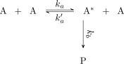
Using steady state approximation: \[ [\mathrm{A}^{*}] = \frac{k_a[\mathrm{A}]^2}{k_b + k_a'[\mathrm{A}]}. \]
6.2. Polymerization
6.2.1. Fraction of Condensed Groups
\[ p := \frac{[\mathrm{A}]_0 - [\mathrm{A}]}{[\mathrm{A}]_0} \] where \( [\mathrm{A}] \) is the concentration of the functional group \( \mathrm{A} \).
6.2.2. Degree of Polymerization
\[ \expval{N} = \frac{[\mathrm{A}]_0}{[\mathrm{A}]} = \frac{1}{1-p}. \] It is the average chain length of a polymer.
6.2.3. Kinetic Chain Length
\[ \lambda := \frac{\text{\# monomer cosumed per volume}}{\text{\# new chain produced}} \]
6.2.4. Stepwise Polymerization
Any two monomer can react.
Each polymer during the reaction has two complementary sites \( \rm A, B \) that is used for reaction. \[ \dv{[\mathrm{A}]}{t} = -k_{\mathrm{r}} [\mathrm{A}]^2. \]
The degree of polymerization grows linearly in time: \[ \expval{N} = 1 + k_{\mathrm{r}}t[\mathrm{A}]_0. \]
6.2.5. Chain Polymerization
Only activated monomer can react.
\[ \schemestart 1/2 In \arrow(--.east){->[$k_i$]}[-90] M \+ \chemfig{\charge{0=\.}{R}} \arrow{->[fast]} \chemfig{\charge{180=\.}{M_1}} \arrow{-U>[M]}[-90] \chemfig{\charge{180=\.}{M_2}} \arrow{->[$k_p$]}[-90] \vdots \arrow{-U>[M]}[-90] \chemfig{\charge{180=\.}{M_n}} \arrow(aa--bb){-U>[\chemfig{\charge{180=\.}{M_m}}]}[180] \chemfig{M_{n+m}} \arrow(@aa--@bb){->[$k_t$]}[180] \arrow(@aa--cc){-U>[\chemfig{\charge{180=\.}{M_m}}][\chemfig{M_m}]} \chemfig{M_n} \arrow(@aa--@cc){->[][$k_t$]} \schemestop \]
The steady state approximation gives: \[ \dv{[\vdot \mathrm{M}]}{t} = 2fk_i[\mathrm{In}] - 2k_t [\vdot \mathrm{M}]^2 = 0 \] where \( [\vdot \mathrm{M}] \) is the concentration of all chains, \( f \) is the fraction of radicals that initiate a chain.
From the approximation the kinetic chain length is: \[ \lambda = \frac{k_p[\vdot \mathrm{M}][\mathrm{M}]}{2k_t[\vdot \mathrm{M}]^2} = \frac{k_p}{\sqrt{fk_ik_t}} \frac{[\mathrm{M}]}{\sqrt{[\mathrm{In}]}}. \] We are using the fact that the activation rate is equal to the termination rate in steady state approximation.
The degree of polymerization is then twice that, because two chain combines in the end \[ \expval{N} = 2\lambda. \]
6.3. Michaelis-Menten Mechanism
\[ \schemestart E \+ S \arrow{<=>[$k_a$][$k_a'$]} \chemfig{E\vdot S} \arrow{->[$k_b$]} P \+ E \schemestop \] \( \rm E \) is for enzyme, \( \rm S \) is for substate, and \( \rm P \) is for product.
6.3.1. Michaelis Constant
\[ K_{\mathrm{M}} := \frac{k_a' + k_b}{k_a} \]
If we assume the steady state, \[ K_{\mathrm{M}} = \frac{[\mathrm{E}][\mathrm{S}]}{[\mathrm{E\vdot S}]} \]
6.3.2. Lineweaver-Burk Plot
We further assume that the substrate is much more than the enzyme, then: \[ [\mathrm{E\vdot S}] = \frac{[\mathrm{E}]_0}{1 + K_{\mathrm{M}}/[\mathrm{S}]_0}. \] This relation can be used to express the rate of production: \[ v = k_b[\mathrm{E\vdot S}] = \frac{k_b[\mathrm{E}]_0}{1 + K_{\mathrm{M}}/[\mathrm{S}]_0}. \] Rearranging this equation, we get the plot of \( 1/v \) as a function of \( 1/[\mathrm{S}]_0 \): \[ \frac{1}{v} = \frac{1}{v_{\rm max}} + \frac{K_{\mathrm{M}}}{v_{\rm max}} \frac{1}{[\mathrm{S}]_0}. \]