Projective Geometry

1. Affine Geometry
2. Homogeneous Coordinate
- 2.1. Homegenization
3. Projective Space
4. Transformations
- 4.1. Affine Transformation
- 4.2. Projective Transformation
  - 4.2.1. One-dimensional Real Projective Transformation
5. Projective Dual
- 5.1. Definition
- 5.2. Dual Thoerems
6. Desargues's Theorem
7. Reference

1. Affine Geometry

Euclidean geometry without the notion of distance and angle.
From the Latin affinis, "connected with".

1.1. Playfair's Axiom

It is the substitute for the Euclid's parallel postulate.

1.1.1. Axiom

Given a line and a point in a plane, at most one line parallel to the line that passes the point exists.

1.2. Affine Transformation

Geometric Transformation that preserves lines and parallelism.
Basically, a combination of reflection, rotation, scaling, translation, shearing, homothety

1.2.1. Homothety

Scaling with respect to a point.

1.2.2. Properties

The number of intersections would not change under covariant affine transformations. See here.

1.3. Affine Space

The plane \(z=1\) in three dimensional space is affine.

1.4. Barycentric Coordinate System

1.4.1. Definition

Given \(n+1\) points \(\{A_i\}_{i=0}^n\) in a \(n\)-dimensional affine space that are affinely independent, the barycentric coordinate \((a_0:\mathord{\dots}: a_n)\) can be constructed, such that: \[ (a_0+\cdots + a_n)\overrightarrow{OP} = a_0\overrightarrow{OA_0} + \cdots +a_n\overrightarrow{OA_n}. \]

1.4.2. Normalized Barycentric Coordinates

Absolute Barycentric Coordinates
- With the additional condition: \[ \sum a_i = 1. \]

2. Homogeneous Coordinate

2.1. Homegenization

It is a process that makes the polynomials homogeneous, that is, every terms having the same degree.
- Introduce a new variable \( \tilde{z} \) and replace \(x = \tilde{x}/\tilde{z}\) and \(y = \tilde{y}/\tilde{z}\).
- It extends the domain of the polynomial by one dimension, of which the original space is a projection, projectivizing the original space as the equivalence classes of the larger space.

3. Projective Space

3.1. Finite Projective Space

3.1.1. Fano Plane

\( \mathrm{PG}(2,2) \)

3.2. Real or Complex Projective Space

It is the quotient space of the vector space over a field by the equivalence relation generated by scalar multiplication.

It can also be seen as a topological space.

3.3. Projective Plane

3.3.1. Definition

A projective plane consists of a set of lines \( L \), a set of points \( P \), and a incidence relation \( \rm I \) with the properties:

Given two distinct points, there is exactly one line incident with both of them.
Given two distinct lines, there is exactly one point incident with both of them.
There are four points such that no line is incident with more than two of them.

3.3.2. Properties

Exists points at infinity, and line at infinity.

3.3.3. Pappian Plane

Projective plane in which Pappus's hexagon theorem is valid is called pappian planes.

4. Transformations

4.1. Affine Transformation

Maps lines to lines.
Parallel lines remain parallel.
Include translations.
See affine transformation

4.2. Projective Transformation

Homography
Parallel lines does not needs to stay parallel.
The two points that lie on every circle (???) #SoME3 - YouTube

4.2.1. One-dimensional Real Projective Transformation

\begin{align*} f\colon x\mapsto \frac{ax + b}{cx +d} = \left( \begin{bmatrix} \tilde{x} \\ \tilde{y} \end{bmatrix} \mapsto \tilde{x}/\tilde{y} \right) \circ \begin{bmatrix} a & b \\ c & d \end{bmatrix} \circ \left( x \mapsto\begin{bmatrix} x \\ 1 \end{bmatrix} \right) \end{align*}

where \( a, b, c, d\in \mathbb{R} \).

The homogenization is canonically a map \( \mathbb{R} \to \mathrm{P}^1(\mathbb{R}) \), and its left inverse (inverse element when multiplied on the left) exists, and right inverse exists on a restricted domain, excluding the point at infinity.

If the inverse of the projective transformation exists, then the inverse of \( f \) exists, on the domain excluding the element which the projective transformation maps to the point at infinity, depending on whether it is left or right inverse:

\begin{equation*} f^{-1}: x \mapsto \frac{dx - b}{-cx + a}. \end{equation*}

Interestingly, if we extend the real function \( f \) into a complex function: \[ f\colon z \mapsto \frac{az + b}{cz + d},\quad a,b,c,d \in\mathbb{C}, \] \( f \) is now a conformal transformation on the complex plane, called the Möbius transformation.

5. Projective Dual

5.1. Definition

For a projective plane \( C = (P, L ,{\rm I}) \) that consists of points \( P \), lines \( L \), and incidence relation \( \rm I \), the dual plane is: \[ C^* = (L, P, {\rm I}^*) \] where \( \rm I^* \) is the converse relation of \( \rm I \).

5.2. Dual Thoerems

Since the real projective plane \(\mathrm{PG}(2,\mathbb{R})\) is self-dual, there exist dual theorems.
Desargues's theorem ↔ Converse of Desargues' Theorem
Pascal's theorem ↔ Brianchon's Theorem
Menelaus's theorem ↔ Ceva's theorem

6. Desargues's Theorem

6.1. Statement

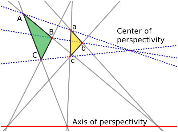
Two triangles are in perspective axially if and only if they are in perspective centrally.
It is true for any projective space defined over a field or division ring, which includes the space in which Pappus's hexagon theorem.

6.2. Proof

The plane is a projection of \(\mathbb{R}^3\), and in \(\mathbb{R}^3\) the plane \(\alpha\) containing \(\triangle abc\) and the plane \(\beta\) containing \(\triangle ABC\) intersect in a line. Furthermore, the plane \(\gamma\) containing \(a, b, A, B\) and the planes \(\alpha\), \(\beta\) intersect in a point that is contained in the intersection of \(\alpha, \beta\).
Projective Geometry 4 Desargues' Theorem Proof - YouTube

6.3. Desarguesian Plane

Projective plane in which Desargues's theorem is true is called Desarguesian plane.
Pappian plane is also a Desarguesian plane.