Units
Table of Contents
- 1. Commensurable
- 2. Conversion Factor
- 3. Common Units
- 4. Centimeter-Gram-Second System of Units
- 5. Natural Units
- 6. Obscure Units
- 7. See Also
- 8. Reference
There is no unit in mathematics in the first place. By assigning units to quantities, you are endowing the quantity a physical significance. Therefore the physicality has to be taken into account thereon.
1. Commensurable
- Two units are commensurable if they can added together.
2. Conversion Factor
- A dimensionless number 1 that is a ratio of two measures.
- e.g. \(1=100\, \mathrm{cm}/1\,\mathrm{m}\)
- For incommensurable units, it depends on the context.
- e.g. \(1=100\, \mathrm{km}/3\,\mathrm{h}\iff 100 \mathrm{km}=3\,\mathrm{h}\)
- Degree, the unit of angle, can be thought of as a conversion factor.
- \[^{\circ} =\frac{\pi}{180}\]
3. Common Units
3.1. SI Units
- International System of Quantities (ISQ)
3.1.1. SI Base Units
| Quantity | Dimension | SI Base Unit | |
|---|---|---|---|
| Length | \(l\) | \(\sf L\) | \(\rm m\) |
| Mass | \(m\) | \(\sf M\) | \(\rm kg\) |
| Time | \(t\) | \(\sf T\) | \(\rm s\) |
| Electric Current | \(I\) | \(\sf I\) | \(\rm A\) |
| Thermodynamic Temperature | \(T\) | \(\sf \Theta\) | \(\rm K\) |
| Amount of Substance | \(n\) | \(\sf N\) | \(\rm mol\) |
| Luminous Intensity | \(I_\mathrm{v}\) | \(\sf J\) | \(\rm cd\) |
3.1.2. SI Derived Units
| Name | Symbol |
|---|---|
| radian | \(\rm rad\) |
| steradian | \(\rm sr\) |
| hertz | \(\rm Hz\) |
| newton | \(\rm N\) |
| pascal | \(\rm Pa\) |
| joule | \(\rm J\) |
| watt | \(\rm W\) |
| coulomb | \(\rm C\) |
| volt | \(\rm V\) |
| farad | \(\rm F\) |
| ohm | \(\Omega\) |
| siemens | \(\rm S\) |
| weber | \(\rm Wb\) |
| tesla | \(\rm T\) |
| henry | \(\rm H\) |
| degree Celsius | \(\rm ^\circ C\) |
| lumen | \(\rm lm\) |
| lux | \(\rm lx\) |
| becquerel | \(\rm Bq\) |
| gray | \(\rm Gy\) |
| sievert | \(\rm Sv\) |
| katal | \(\rm kat\) |
| Unit | |
|---|---|
| Electric Field | \(\rm V/m\) |
| Permittivity | \(\rm F/m\) |
3.1.3. Prefixes
| Name | Symbol | Base 10 Factor |
|---|---|---|
| quetta | \(\rm Q\) | \(10^{30}\) |
| ronna | \(\rm R\) | \(10^{27}\) |
| yotta | \(\rm Y\) | \(10^{24}\) |
| zetta | \(\rm Z\) | \(10^{21}\) |
| exa | \(\rm E\) | \(10^{18}\) |
| peta | \(\rm P\) | \(10^{15}\) |
| tera | \(\rm T\) | \(10^{12}\) |
| giga | \(\rm G\) | \(10^{9}\) |
| mega | \(\rm M\) | \(10^{6}\) |
| kilo | \(\rm k\) | \(10^3\) |
| hecto | \(\rm h\) | \(10^2\) |
| deca | \(\rm da\) | \(10^1\) |
| \(\text{--}\) | \(\text{--}\) | \(1\) |
| deci | \(\rm d\) | \(10^{-1}\) |
| centi | \(\rm c\) | \(10^{-2}\) |
| milli | \(\rm m\) | \(10^{-3}\) |
| micro | μ | \(10^{-6}\) |
| nano | \(\rm n\) | \(10^{-9}\) |
| pico | \(\rm p\) | \(10^{-12}\) |
| femto | \(\rm f\) | \(10^{-15}\) |
| atto | \(\rm a\) | \(10^{-18}\) |
| zepto | \(\rm z\) | \(10^{-21}\) |
| yocto | \(\rm y\) | \(10^{-24}\) |
| ronto | \(\rm r\) | \(10^{-27}\) |
| quecto | \(\rm q\) | \(10^{-30}\) |
3.2. Avoirdupois
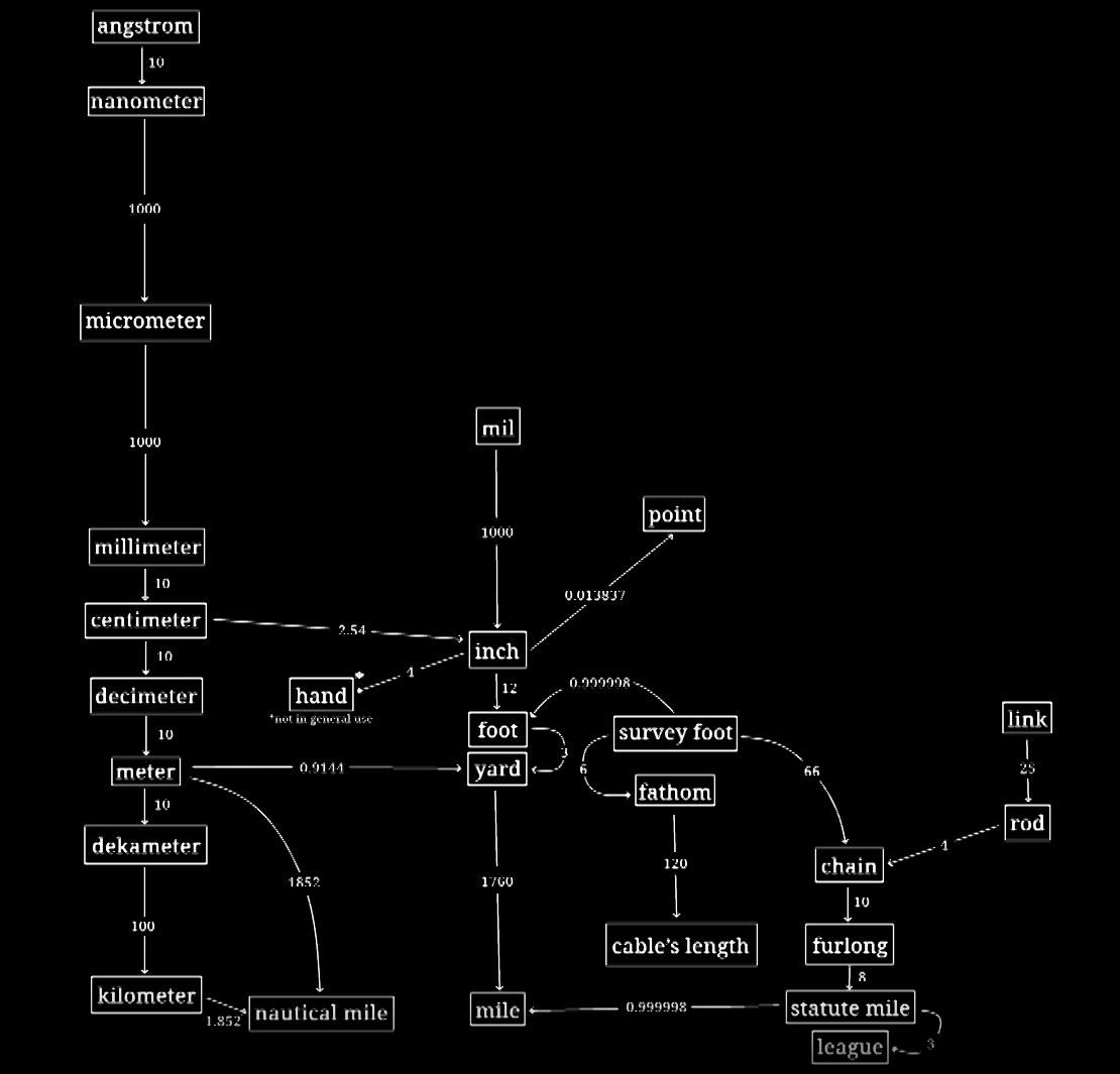
- a defense of the imperial measurement system - YouTube
- Imperial Units
- US Customary Units
- Yard-Pound System
- Everyday use in USA1
3.2.1. Yard
- 0.9144 m
3.2.2. Mile
- 1760 yards.
- It originated from the different unit system, the Roman one.
3.2.3. Pound
- 0.454 kg
3.2.4. Ounce
- oz, oz.
- Alchemical symbol for an ounce ℥, and half an ounce 🝳.
- 28.34 g
- 1/16 avoirdupois pound
3.2.5. Fluid Ounce
- fl oz, fl. oz.
- US Customary: 29.57 mL
- US Food Labelling: 30 mL
3.2.6. Point
- The definition may vary.
3.2.6.1. DTP
- desktop publishing point
- 1/72 of an inch, 1/12 of a pica.
- 0.3528 mm.
3.2.6.2. New Didot Point
nd- 3/8 mm, or 0.375 mm.
3.2.6.3. American Point
- American point system
- 1/72.27 of an inch,
- TeX point 0.351 459 80 mm
- Point (typography) - Wikipedia
3.2.7. Horsepower
- Watt determined that a horse could turn a mill wheel 144 times in an hour, or 2.4 times in a minute. The wheel was 12 feet (3.7 m) in radius, and Watt judged that the horse could pull with a force of 180 pounds-force (800 N).
- \[ 1\,\mathrm{hp} = 180\,\mathrm{lbf}\cdot 2.4\,\mathrm{turn/min}\cdot (2\pi\cdot 12)\,\mathrm{ft/turn} = 32,572\,\mathrm{ft\,lbf/min} \]
3.2.7.1. Imperial Horsepower
- \(1\,\mathrm{hp} = 745.7\,\mathrm{W}\)
3.2.7.2. Metric Horsepower
- 735.5 W
3.3. Level
3.3.1. Decibel
- dB (base quantity) is the unit of the level.
\[ L = 10 \log \frac{Q}{Q_0}\ \mathrm{dB} \]
- A reference unit can be provided so that the quantity have a unit.
3.3.1.1. dBm
- decibel-milliwatts
3.3.1.2. Root-Power Quantity
- Often used for voltage.
- 20 is used.
3.3.2. Neper
- Np
- natural logarithm is used.
3.4. Information
3.4.1. Shannon
- Log 2 of probability
3.4.2. Nat
- Natural log of probability
4. Centimeter-Gram-Second System of Units
- CGS Units, CGS, cgs
4.1. In Mechanics
| Quantity | Quantity Symbol | Unit Name | Unit Symbol | Description |
|---|---|---|---|---|
| Acceleration | \(a\) | gal(galileo) | \(\rm Gal\) | |
| Force | \(F\) | dyne | \(\rm dyn\) | From Greek, δύναμις, "power" |
| Energy | \(E\) | erg | \(\rm erg\) | From Greek, ἔργον, "work" |
| Pressure | \(p\) | barye | \(\rm Ba\) | |
| Dynamic Viscosity | \(\mu\) | poise | \(\rm P\) | \(\rm cP\) is more common |
| Kinematic Viscosity | \(\nu\) | stokes | \(\rm St\) | |
| Wavenumber | \(k\) | kayser | \(\rm K\) |
4.2. In Electromagnetism
4.2.1. Electrostatic Units
- ESU, CGS-ESU
4.2.1.1. Statcoulomb
- \(\rm statC\)
- 4.2.3.3.1, esu charge
- ESU has smaller charge units and larger charge components.
- a statcoulomb is equivalent to \( c \) times the abcoulomb.
4.2.1.2. Stattesla
- \(\rm statT\)
- It does not include the factor of \(c\), compared to 4.2.3.
- \[ \mathbf{B}^{\sf ESU} := \sqrt{4\pi\varepsilon_0}\,\mathbf{B}^{\sf SI} \]
- \[ \mathbf{F} = q^{\sf ESU}\mathbf{v}\times \mathbf{B}^{\sf ESU} \]
4.2.2. Electromagnetic Units
- EMU, CGS-EMU
4.2.2.1. Abampere
- Biot, emu current
- \(\rm abA\), \(\rm Bi\)
- \[ I^{\sf EMU} := \sqrt{\frac{\mu_0}{4\pi}} I^{\sf SI} = \frac{I^{\sf SI}}{c\sqrt{4\pi\varepsilon_0}} \]
- For currents through two parallel conductors of infinite length, \[ \frac{F}{2} =\frac{I_1^{\sf EMU}I_2^{\sf EMU}}{r} \]
- \[ \mathbf{B}^{\sf EMU} = \frac{I^{\sf EMU}d\mathbf{l}\times \mathbf{\hat{r}}}{r^2} \]
4.2.2.2. Gauss
- \[ \mathbf{B}^{\sf EMU} = c\sqrt{4\pi\varepsilon_0}\,\mathbf{B}^{\sf SI} \]
- EMU has smaller field units and larger field components.
- a gauss is equivalent to e\( c \) times the 4.2.1.2.
4.2.3. Gaussian Units
- CGS-Gaussian
- Follows ESU for electricity and EMU for magnetism.
- Gaussian Unit System, Gaussian-CGS Units, CGS Units
Conversion factors can be absorbed into the unit itself.
4.2.3.1. Quantities
4.2.3.1.1. Charge
- \[ q^\mathrm{G} := \frac{q^\mathrm{I}}{\sqrt{4\pi\varepsilon_0}} \]
- It is so defined to simplify the Coulomb's law: \[ F = \frac{q_1^\mathrm{G}q_2^\mathrm{G}}{r^2} \]
- The point is to express charge entirely from mass, length, and
time:
- \[ [\text{charge}] = \sf M^{1/2}L^{3/2}T^{-1}. \]
4.2.3.1.2. Electric Field
- \[ \mathbf{E}^\text{G} := \sqrt{4\pi\varepsilon_0}\,\mathbf{E}^\text{I} \]
- Motivatied by:
- \[ \mathbf{E}^\mathrm{G} = \frac{q^\text{G}}{r^2}\mathbf{\hat{r}} = \frac{\mathbf{F}}{q^\mathrm{G}}. \]
4.2.3.1.3. Magnetic Field
- It is defined to have the same dimension as the electric field.
- The factor of \(c\) is absorbed into the unit of magnetic field.
- \[ \mathbf{B}^\mathrm{G} = c\sqrt{4\pi\varepsilon_0}\,\mathbf{B}^\mathrm{I} = \sqrt{\frac{4\pi}{\mu_0}}\,\mathbf{B}^\mathrm{I} \]
4.2.3.2. Implication
- Equations related to electromagnetism are adjusted accordingly.
- \[ \mathbf{F} = q^\mathrm{G}\left(\mathbf{E}^\mathrm{G} + \frac{1}{c}\mathbf{v}\times \mathbf{B}^\mathrm{G}\right) \]
- \[ \rho^\text{G} = \frac{\rho^\text{I}}{\sqrt{4\pi\varepsilon_0}} \]
- \[ I^\mathrm{G} = \frac{I^\mathrm{I}}{\sqrt{4\pi\varepsilon_0}} \]
4.2.3.2.1. Maxwell's Equations
- \[ \nabla\cdot \mathbf{E}^\text{G} = 4\pi \rho^\text{G} \]
- \[ \nabla \cdot \mathbf{B}^\mathrm{G} = 0 \]
- \[ \nabla\times \mathbf{E}^\mathrm{G} + \frac{1}{c} \frac{\partial \mathbf{B}^\mathrm{G}}{\partial t} = 0 \]
- \[ \nabla\times \mathbf{B}^\mathrm{G} - \frac{1}{c}\frac{\partial \mathbf{E}^\mathbf{G}}{\partial t} = \frac{4\pi}{c}\mathbf{J}^\mathrm{G} \]
4.2.3.3. Units
- Physicist's use of Gaussian units does not care too much whether it
is cgs or not:
- \[ \rm 1\ statC = 10^{-\frac{9}{2}}\ kg^{1/2}m^{3/2}s^{-1} = 10^{-\frac{9}{2}}\ C^G \]
- \[ \rm C^G = \frac{C}{\sqrt{4\pi\varepsilon_0}} \]
4.2.3.3.1. Franklin
- Unit of electric charge
- \[ \rm Fr = cm^{3/2}g^{1/2}s^{-1} \]
- Equivalent to the standard unit is the electrostatic unit: \[
1\ \text{statC} := 1\ {\rm g^{1/2} cm^{3/2} s^{-1}}
\]
- \[ \rm dyn = g\,cm\,s^{-2} = \frac{statC^2}{cm^2} \]
4.2.3.3.2. Gauss
- Unit of electric field or magnetic B field
- Hence, Gaussian Units
- \[ \rm G = cm^{-1/2}g^{1/2}s^{-1} = 10^{-\frac{1}{2}}\ m^{-1/2}kg^{1/2}s^{-1} \]
- Note that the conversion factor from the SI is nicely canceled:
- \[ \frac{\mathbf{B}^{\mathrm{G}}}{\mathbf{B}^\mathrm{I}} = \sqrt{\frac{4\pi}{\mu_0}} \approx \sqrt{\frac{4\pi}{4\pi\times 10^{-7}\ \mathrm{N/A^2}}} = 10^{\frac{7}{2}}\rm\ N^{-1/2}A = \frac{10^4\ G}{1\ T} \]
5. Natural Units
5.1. Planck Units
5.1.1. Quantities
- Every quantities are scaled by the factor of plank quantities, yielding dimensionless quantities that corresponds to the normal quantities.
| Name | Expression |
|---|---|
| Plank length | \(l_\text{P} = \sqrt{\dfrac{\hbar G}{c^3}}\) |
| Plank mass | \(m_\text{P} = \sqrt{\dfrac{\hbar c}{G}}\) |
| Plank time | \(t_\text{P} = \sqrt{\dfrac{\hbar G}{c^5}}\) |
| Plank temperature | \(T_\text{P} = \sqrt{\dfrac{\hbar c^5}{Gk_\text{B}^2}}\) |
| Plank charge | \(q_\text{P} = \sqrt{4\pi\varepsilon_0\hbar c}\ (k_\text{B} = 1)\quad\text{or}\quad \sqrt{\varepsilon_0\hbar c}\ (\varepsilon_0 = 1)\) |
5.1.2. Units
- The units can be thought of as the ratio to the Plank quantities.
- e.g.
- \[ [\text{length}] = \frac{\rm m}{l_\text{P}} \]
- e.g.
5.1.3. Implications
- The effect is equivalent to setting \(c = G = \hbar = k_\text{B} = 1\)
- \[ F = \frac{m_1m_2}{r^2} \]
5.2. Heaviside-Lorentz Units
5.2.1. Quantities
- Only the \(\varepsilon_0\) is removed compared to the Gaussian units.
- \[ q^{\sf HL} := \frac{q^{\sf SI}}{\sqrt{\varepsilon_0}} \]
- \[ \mathbf{E}^{\sf HL} := \sqrt{\varepsilon_0}\,\mathbf{E}^{\sf SI} \]
- \[ \mathbf{B}^{\sf HL} := c\sqrt{\varepsilon_0}\,\mathbf{B}^{\sf SI} = \frac{1}{\sqrt{\mu_0}}\mathbf{B}^{\sf SI} \]
5.3. Atomic Units
5.3.1. Quantities
- Similar to Planck units, but set \(\hbar = e = m_\text{e} = 4\pi\varepsilon_0 = 1\).
6. Obscure Units
6.1. Airwatt
\( \rm AW, airW \)
The product of suction pressure (in Pascal) and air flow rate (in cubic meter per second): \[ P = p\cdot Q. \]
7. See Also
- How To Multiply Dog × Tree?! A Dimensional Analysis Primer - YouTube
- Anything is unit
- Cursed Units 2: Curseder Units - YouTube
- Radian
- \[ \rm rad = \frac{arclength}{radius} \]
- pH
- \[ \rm pH = -\log\left(\frac{molar\ concentration}{1\ mol/L}\right) \]
- Radian
- \(\stackrel{\frown}{=}\), ≘ U+2258
- 'Corresponds'
8. Reference
- International System of Units - Wikipedia
- International System of Quantities - Wikipedia
- SI derived unit - Wikipedia
- Decibel - Wikipedia
- dBm - Wikipedia
- Shannon (unit) - Wikipedia
- International System of Units - Wikipedia
- International System of Quantities - Wikipedia
- SI derived unit - Wikipedia
- Centimetre–gram–second system of units - Wikipedia
- Gaussian units - Wikipedia
- Planck units - Wikipedia
- Heaviside–Lorentz units - Wikipedia
- Atomic units - Wikipedia
- Airwatt - Wikipedia