Linear Algebra
Table of Contents
- 1. Vector
- 2. Vector Space
- 3. Linear Independence
- 4. Vector Identites
- 5. Matrix
- 5.1. Size
- 5.2. Square Matrix
- 5.2.1. Identity Matrix
- 5.2.2. Elementary Matrix
- 5.2.3. Permutation Matrix
- 5.2.4. Projection Matrix
- 5.2.5. Nilpotent Matrix
- 5.2.6. Diagonal Matrix
- 5.2.7. Triangular Matrix
- 5.2.8. Strictly Triangular Matrix
- 5.2.9. Hessenberg Matrix
- 5.2.10. Definite Matrix
- 5.2.11. Symmetric Matrix
- 5.2.12. Skew-Symmetric Matrix
- 5.2.13. Hermitian Matrix
- 5.2.14. Orthogonal Matrix
- 5.2.15. Special Orthogonal Matrix
- 5.2.16. Unitary Matrix
- 5.2.17. Special Unitary Matrix
- 5.2.18. Normal Matrix
- 5.2.19. Complex Diagonalizable Matrix
- 5.3. Rectangular Matrix
- 5.4. Minor
- 5.5. Cofactor
- 5.6. Invertible Matrix
- 5.7. Pseudo Inverse Matrix
- 6. Products
- 7. Associated Spaces
- 8. Rank
- 9. Determinant
- 10. Trace
- 11. Rotation Matrix
- 12. Cramer's Rule
- 13. Rouché-Capelli Theorem
- 14. Matrix Operations
- 15. Normal Equation
- 16. Spectral Theorem
- 17. Characteristic Polynomial
- 18. Minimal Polynomial
- 19. Rayleigh Quotient
- 20. Gram-Schmidt Process
- 21. Gram Matrix
- 22. Block Matrix
- 23. Vectorization
- 24. Matrix Decomposition
- 24.1. LU Decomposition
- 24.2. QR Decomposition
- 24.3. Spectral Decomposition
- 24.4. Schur Decomposition
- 24.5. Jordan Normal Form
- 24.6. Jordan-Chevalley Decomposition
- 24.7. Canonical Forms
- 24.8. Singular Value Decomposition
- 24.9. Choleskey Decomposition
- 24.10. Polar Decomposition
- 24.11. Simultaneous Diagonalization by Congruence
- 25. Matrix Relations
- 26. Sylvester's Law of Inertia
- 27. Matrix Norms
- 28. Pfaffian
- 29. Matrix Order
- 30. Principal Square Root
- 31. Null Vector
- 32. Matrix Pencil
- 33. References
1. Vector
- Vector is a list of numbers
- Vector is represented by an arrow.
- Vector is an element of a vector space
2. Vector Space
- Linear Space
Vector space is a triplet \((V, +, \cdot)\) over a field \(K\), a set \( V \), and two linear operations \( +: V\times V \to V\)(vector addition) and \( \cdot: K\times V \to V \)(scalar multiplication)
2.1. Definition
- Associativity of Vector Addition
- Commutativity of Vector Addition
- Identity Element of Vector Addition
- Inverse Elements of Vector Addition
- Compatibility of Scalar Multiplication with Field Multiplication
- Identity Element of Scalar Multiplication
- Distributivity of Scalar Multiplication with respect to Vector Addition
- Distributivity of Scalar Multiplication with respect to Field Addition
2.2. Basis
Set of linearly independent vectors that spans the entire vector space.
2.2.1. Standard Basis
- Natural Basis, Canonical Basis
Depending on the construction of vector space, there might exists obvious basis.
2.3. Coordinate Space
- Coordinate Vector Space
\(n\)-tuples of elements of a field \(F\) forms a coordinate vector space \(F^n\), equipped with the canonical addition and scalar multiplication.
3. Linear Independence
3.1. Definition
3.1.1. For Finite Set of Vectors
The set of vectors \( \{ \mathbf{v}_1, \dots, \mathbf{v}_k \} \) is said to be linearly independent if \[ a_1\mathbf{v}_1 + a_2\mathbf{v}_2 + \cdots + a_k\mathbf{v}_k = \mathbf{0} \implies a_1 = a_2 = \cdots = a_k = 0 \] where \( a_i \) are the elements of the field associated with the underlying vector space.
3.1.2. For Infinite Set of Vectors
- If every nonempty finite subset of vectors is linearly independent.
3.2. Dimension
The dimension of a vector space \( V \) is the size of the largest linearly independent subset, the basis. Formally, \[ \dim(V) = \mathop{\mathrm{arg\ max}}_k \left( \{ v_1, \dots, v_k \} \text{ linearly independent} \colon v_1,\dots, v_k \in V\right). \]
3.3. Matroid
Generalization of the linearly independent subset.
4. Vector Identites
4.1. Lagrange Identity
\[ (a\times b)\cdot (c\times d) = (a\cdot c)(b\cdot d)-(b\cdot c)(a\cdot d). \]
4.2. Grassmann Identity
\[ a\times (b\times c) = (a\cdot c)b - (a\cdot b)c. \]
4.3. Jacobi Identity
\[ a\times (b\times c) + b\times (c\times a) + c\times (a\times b) = 0. \] Equivalently, the cross product has the product rule: \[ a\times (b\times c) = (a\times b)\times c + b\times (a\times c). \]
5. Matrix
- Matrices do transformation on a vector space.
- Set of Matrices with operation defined on them forms a group.
- Name of the transformations and groups follows the name of the matrix.
5.1. Size
- Dimension
The dimension of the matrix. e.g. 2 by 2 matrix.
5.2. Square Matrix
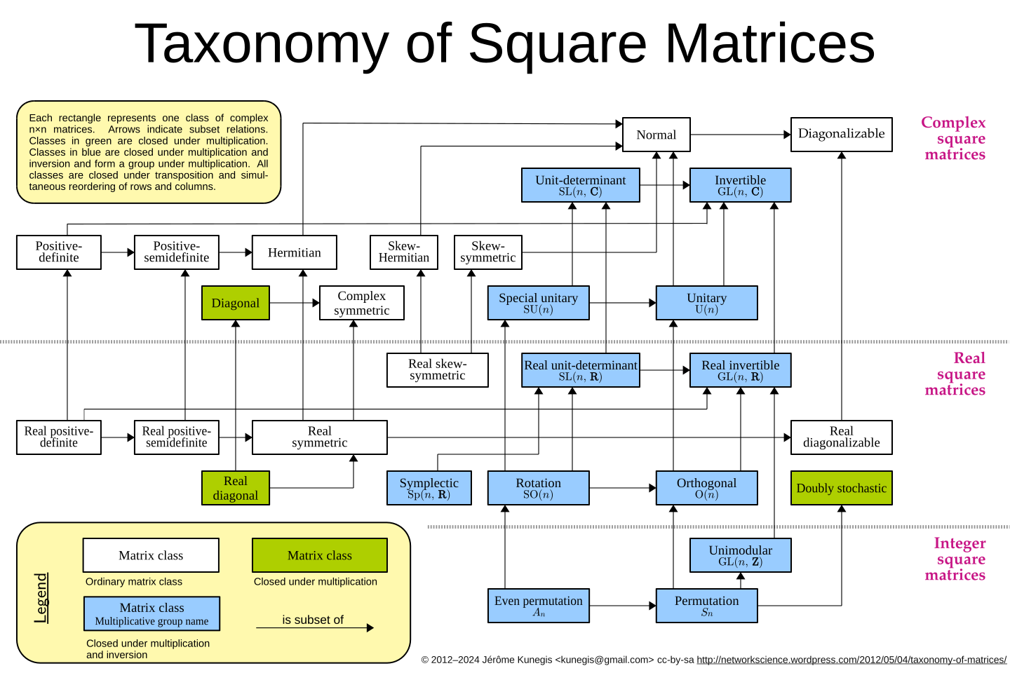
Figure 1: taxonomy
5.2.1. Identity Matrix
- No rectangular identity.
5.2.2. Elementary Matrix
- A matrix which differs from the identity matrix by one of the elementary row operations, which in turn represents that single row operation by multiplying on the left.
- Elementary matrix - Wikipedia
5.2.3. Permutation Matrix
5.2.3.1. Properties
- \[ P^2 = I \]
5.2.4. Projection Matrix
5.2.4.1. Definition
- \[ P^2 = P \]
5.2.5. Nilpotent Matrix
\[ \exists k \in \mathbb{N}, N^k = 0. \] The smallest such \( k \) is called the index of \( N \).
5.2.6. Diagonal Matrix
5.2.6.1. Definition
- All entries are zero, except along the main diagonal.
5.2.6.2. Properties
- \[ D^{\rm T} = D \]
5.2.7. Triangular Matrix
5.2.8. Strictly Triangular Matrix
Strictly upper (or lower) triangular matrix \( A \) is a matrix such that \( A_{ij} = 0 \) if \( i\ge j \) (or \( i\le j\) ).
5.2.8.1. Properties
It is nilpotent, since when exponentiated by the number of rows, it yields zero matrix.
5.2.9. Hessenberg Matrix
Zeros above the superdiagonal or below the subdiagonal.
5.2.10. Definite Matrix
5.2.10.1. Definition
- \(\mathbf{x}^{\rm \dagger}M\mathbf{x}\) is definite .
5.2.10.2. Equivalent Statements
- \(M\) is positive-definite.
- \(M\) is congruent with a diagonal matrix with positive real entries.
- \(M\) is Hermitian and all its eigenvalues are real and positive.
- \(M\) is Hermitian and all its leading principal minors are positive.
- There exists an invertible matrix \(B\) with conjugate transpose \(B^*\) such that \(M=B^*B\).
5.2.11. Symmetric Matrix
5.2.11.1. Definition
- \[ S = S^{\rm T} \]
5.2.11.2. Properties
- Its eigen vectors are orthogonal.
- The singular value decomposition is of the form:
\[
S = U\Sigma U^{-1}
\]
- which is also the 24.3.
- The symmetry is preserved under the operation \(M^{\rm T}(\cdot )M\).
5.2.11.3. Construction
- For any matrix \(M\):
- \(MM^{\rm T}\)
- \(M + M^{\rm T}\)
5.2.12. Skew-Symmetric Matrix
5.2.12.1. Definition
- \[ S = -S^{\rm T} \]
5.2.12.2. Construction
- For any matrix \(M\):
- \(M-M^{\rm T}\)
- The skew-symmetry is also preserved under the operation \(M^{\rm T}(\cdot )M\).
5.2.12.3. Symplectic Matrix
- \(2n\times 2n\) matrix \(M\) with real entries that satisfies: \[ M^\top \Omega M = \Omega \] where \(\Omega\) is a fixed \(2n\times 2n\) nonsigular, skew-symmetric matrix.
5.2.13. Hermitian Matrix
5.2.13.1. Definition
- \[ H = H^\dagger \]
- It is an adjoint matrix with respect to the inner product.
- Note that conjugate transpose of a 2 by 2 matrix is just transpose of the corresponding 4 by 4 matrix.
For a real symmetric matrix \(S\) and a real skew-symmetric matrix \(A\): \[ aS + biA \] is Hermitian.
5.2.14. Orthogonal Matrix
- It is the matrix that preserves the magnitudes of vectors.
- It contains rotations and reflections.
5.2.14.1. Definition
- A real square matrix whose columns and rows are orthonormal vectors.
- \[ Q^{\rm T} = Q^{-1} \]
5.2.14.2. Properties
- \[
QQ^{\rm T} = Q^{\rm T}Q = I.
\]
- Note that this means that the dot products of the column or row vectors are given by the .
- \(Q^{\rm T}\) is also orthogonal.
5.2.15. Special Orthogonal Matrix
5.2.15.1. Definition
- Orthogonal matrix with determinant of 1.
5.2.16. Unitary Matrix
5.2.16.1. Definition
- \[ U^\dagger = U^{-1} \]
5.2.16.2. Properties
- Its determinant is a complex number whose magnitude is 1, i.e. \(e^{i\theta}\).
5.2.17. Special Unitary Matrix
5.2.17.1. Definition
- Unitary matrix whose determinant is 1.
5.2.17.2. Properties
- It can be obtained by multiplying a unitary matrix with the square root of its determinant.
5.2.18. Normal Matrix
5.2.18.1. Definition
- It commutes with its conjugate transpose
- \[ A^\dagger A =AA^\dagger \]
5.2.19. Complex Diagonalizable Matrix
- How to "diagonally" think about rotations. - YouTube
- Orthogonal matrix is complex diagonalizable
- See infinite groups
5.3. Rectangular Matrix
- Matrix with \(n\) rows and \(m\) columns.
5.4. Minor
- Determinant of a square submatrix.
5.4.1. n-th Minor
- First Minors of a square matrix \( A \) are the determinants of submatrices of \( A \) with one row and one column removed.
- n-th minors are with n rows and n columns removed.
5.4.2. Principal Minor
- The row indices \( I \) and column indices \( J \) of the original matrix that are used in minor is the same \( I = J \).
5.4.3. Leading Principal Minor
- The square upper-left submatrix.
5.5. Cofactor
5.5.1. Definition
\[ C_{ij} = (-1)^{i+j} M_{ij} \] where \( M_{ij} \) is the first minor with \( i\)-th row and \(j\)-th column removed.
5.5.2. Cofactor Matrix
Cofactor matrix of a matrix \( A \) is the matrix with its \( i,j \) entry is the cofactor \( C_{ij} \) of \( A \).
5.6. Invertible Matrix
- Nonsingular Matrix, Nondegenerate Matrix
- Square matrix that is not invertible is called singular or degenerate.
5.6.1. Definition
An \(m\times n\) matrix \(A\) over a field \(K\) is called invertible if: \[ \exists B\in K^{n\times m}, AB = I_m\land BA = I_n. \] That is, both left inverse and right inverse exists and they are the same, in which case it is called the inverse matrix.
5.6.2. Properties
- It is necessary that \(m=n\).
- Inverse matrix can be obtained from the cofactor matrix \( C \) with: \[ A^{-1} = \frac{1}{\det A} C^{\rm T} \]
5.6.3. Inverse Matrix Theorem
- Matrix Inversion Theorem
5.6.3.1. Statement
- For a square matrix \(A\) over a field \(K\), the following
statements are equivalent:
- \(A\) is invertible
- \(\det A \neq 0\)
- \(A\) has full rank
- \(A\) is bijective
- \(\ker A = \{0\}\)
- Eigenvalues of \(A\) are nonzero
5.7. Pseudo Inverse Matrix
pinv(A)in Matlab.
5.7.1. Left Inverse
5.7.1.1. Definition
For an \(n\times m\) matrix \(A\), if it is full column rank, that is, \(\mathrm{rank}(A) = m \le n\), the left inverse always exists and there are many, but the best one that minimizes the error is \[ A_\text{left}^{-1} = ( A^TA)^{-1}A^T. \]
Notice that \[ A^{-1}_\text{left}A = I_n \] \((A^\top A)^{-1}\) is always possible, because \(A^\top A\) is an \(n\times n\) matrix with full rank.
This matrix exactly corresponds to normal equation.
5.7.1.2. Pseudo Inverse
- If it is used in the opposite order: \[ AA_\text{left}^{-1} = A(A^\top A)^{-1} A^\top \]
- It is not an identity matrix, but a projection matrix onto the column space.
- It is used as a pseudo inverse.
5.7.1.3. Derivation
- Least Squares Formula PROOF - YouTube
- We want to invert \(\mathbf{y}\), but it is not possible because it is outside of the column space.
- So instead, we want at least to find: \[ \operatorname*{argmin}_\mathbf{x}\Vert A\mathbf{x}-\mathbf{y}\Vert \]
- By Hilbert projection theorem, there exists a vector \(\hat{\mathbf{x}}\) that satisfies the condition above.
- By orthogonality of column vectors \(A^\top\) and \(A\hat{\mathbf{x}}-\mathbf{y}\), \[ A^\top(A\hat{\mathbf{x}}-\mathbf{y})=\mathbf{0} \]
- therefore, if \(A^\top A\) is invertible, we have \[ \hat{\mathbf{x}}=( A^\top A)^{-1}A^\top\mathbf{y} \]
5.7.2. Right Inverse
5.7.2.1. Definition
- For an \(n\times m\) matrix \(A\) with full row rank, that is, \(\mathrm{rank}(A) = n \le m\),
- The best right inverse is \[ A_\text{right}^{-1} = A^{\top}(AA^\top)^{-1} \]
- Notice \[ AA^{-1}_\text{right} = I_m \]
- and the inverse of \(AA^\top\) always exists because it is an \(m\times m\) matrix with full rank.
- It can also be used as a pseudo inverse matrix on the left.
5.7.3. Pseudo Inverse
- Pseudo inverse matrix \(A^+\) is a matrix satisfying:
\[
\forall v \in \text{rowspace}(A), A^+Av = v.
\]
- In the case of left inverse the kernel was trivial and the cokernel was nontrivial, and in the case of right inverse the kernel was nontrivial and the cokernel was trivial.
- In general, for a matrix with nontrivial kernel and nontrivial
cokernel, pseudo inverse can be calculated using the singular value decomposition:
\[
A = U\Sigma V^\top \implies A^+ = V\Sigma^+ U^\top
\]
- where \(\sigma^+\) is the diagonal matrix with reciprocal entries, with zeroes untact.
6. Products
6.1. Dot Product
- Scalar Product, Inner Product(🤦♂️), 스칼라곱, 점곱, 내적
- Dot product is proportional to how similar two objects is.
6.1.1. Real Dot Product
\[ \mathbf{x}\cdot \mathbf{y} := \sum_i x_iy_i \]
6.1.2. Complex Dot Product
For two complex vectors \(\mathbf{u}, \mathbf{v}\) dot product is defined as, \[ \mathbf{u}\cdot\mathbf{v}= \sum_i u_i^*v_i \] which gives larger real parts if they are similar in phase.
6.2. Cross Product
6.2.1. Definition
\[ \mathbf{a}\times\mathbf{b}=|a||b||\sin\theta|\hat{a}\times\hat{b} \] where \(\hat{a}\times\hat{b}\) is determined by the right hand rule.
6.2.2. Properties
\[ |\mathbf{a}\times\mathbf{b}|^2=\mathrm{vec}(\mathbf{a}\mathbf{a}^\mathrm{T})\cdot \mathrm{vec}(\mathrm{adj}(\mathbf{b}\mathbf{b}^\mathrm{T})) \] Frobenius product with the Adjugate matrix.
Vectorization \( \mathrm{vec} \) stacks the column vectors of given matrix into a vector.
6.3. Scalar Multiplication
6.4. Matrix-Vector Product
7. Associated Spaces
7.1. Row Space
- \( \mathrm{R}(A) = \mathrm{C}(A^{\rm T}) \)
- The span of the row vectors.
7.2. Null Space
- \( \mathrm{N}(A) \)
- Kernel, \( \ker(A) \)
- The set of null vectors: \( A\mathbf{v} = \mathbf{0} \) .
- The row space and the null space are orthogonal.
- The dimension of the null space is called the nullity.
7.3. Column Space
- \( \mathrm{C}(A) \)
- The span of the column vectors.
7.4. Left Null Space
- \( \mathrm{N}(A^{\rm T}) \)
- Cokernel, \( \mathrm{coker}(A) \)
- The column space and the left null space are orthogonal.
7.5. Eigenspace
- \( \ker(A-\lambda I) \) where \( \lambda \) is one of the eigenvalues.
8. Rank
- The dimension of the row space, which is the dimension of the column space.
- Its also the number of singular values with the corresponding singular vectors multiplied together after # Singular Value Decomposition.
8.1. Rank-Nullity Theorem
8.1.1. Statement
For a linear transformation \(T\colon V\to W\) with finite dimensional vector space \(V\), \[ \mathrm{rank}(T) + \mathrm{nullity}(T) = \dim(V) \] In other words, \[ \dim(\mathrm{im}\,T) + \dim(\mathrm{ker}\,T) = \dim(\mathrm{dom}\,T) \]
8.1.2. Proof By Splitting Lemma
For a short exact sequence \[ 0 \to \mathrm{ker}\,T \hookrightarrow V \xrightarrow{T} \mathrm{im}\,T \to 0, \] by the splitting lemma, \[ \mathrm{ker}\,T \oplus \mathrm{im}\,T \cong V. \]
8.1.3. Fundamental Theorem of Linear Algebra
For a linear transformation \(T\colon V \to W\) with two finite dimensional space \(V, W\), \[ \dim(\mathrm{im}\,T) + \dim(\mathrm{ker}\,T) = \dim(\mathrm{dom}\,T)\\ \dim(\mathrm{im}\,T) + \dim(\mathrm{coker}\,T) = \dim(\mathrm{codom}\,T) \] where \(\mathrm{codom}\, T := W/\mathrm{im}\, T\).
9. Determinant
9.1. Properties
- It is the scaling factor of a \(n\)-dimensional parallelepiped.
- It is a homogeneous function. \(\det(cA) = c^n\det(A)\) for an \(n\times n\) matrix \(A\).
9.2. Leibniz Formula for Determinants
- The determinant of a square matrix \(A\) is:
\[
\det(A) = \sum_{\tau\in S_n}\operatorname{sgn}(\tau)\prod_{i=1}^n a_{i\tau(i)} = \sum_{\sigma\in S_n}\operatorname{sgn}(\sigma)\prod_{j=1}^n a_{\sigma(j)j}
\]
where \(S_n\) is the permutation group
group.
- Alternatively, using the Levi-Civita symbol and the Einstein summation notation: \[ \det(A) = \varepsilon_{i_1\dots i_n} a_{1i_1} \cdots a_{ni_n}. \]
9.3. Laplace Expansion
- Cofactor Expansion
9.3.1. Definition
- The determinant of an square matrix \(A\) is the sum of \(a_{ij}C_{ij}\) in along any row or column: \[ \det(A) = \sum_{i=1}^na_{ij}C_{ij} = \sum_{j=1}^na_{ij}C_{ij} \] where \(C_{ij}\) are the cofactors.
9.4. Properties
- \(\det(A) = \det(A^\top)\)
- The determinant of the transpose is the reciprocal of the area of one gridbox: \(1/\det(A)\).
- \(\det(AB) = \det(A)\det(B)\)
- \(\det(A) = 1/\det(A^{-1})\)
9.5. Of Outermorphism
- Given a linear transformation \(f: V\to V\), its outermorphism extension \(f: \wedge V \to \wedge V\) is defined to satisfy: \[ f(a\wedge b) = f(a) \wedge f(b). \]
- Then the determinant of the outermorphism \(f\) is given by: \[ \det(f) = f(I)I^{-1}. \]
- Determinants in Geometric Algebra - YouTube
10. Trace
10.1. Definition
- \[ \operatorname{tr}\mathbf{A} = \sum_{i=1}^n a_{ii} \]
10.2. Interpretation
- Trace is the divergence of the vector field \(\mathbf{Ax}\).1
- \[ \mathrm{tr}\mathbf{A} = \nabla\cdot (\mathbf{Ax}) \]
- The sum of the eigenvalues.
10.3. Properties
- \(\nabla \operatorname{tr}\mathbf{X} = \mathbf{I}\)
- \(\nabla\) is the gradient.
- Basis-independent
- \(\mathrm{tr}(a\mathbf{A} + b\mathbf{B}) = a\mathrm{tr}(\mathbf{A}) + b\mathrm{tr}(\mathbf{B})\)
- \(\mathrm{tr}(\mathbf{AB}) = \mathrm{tr}(\mathbf{BA})\)
- \(\mathrm{tr}(\mathbf{A}^{\mathsf{T}}) = \mathrm{tr}(\mathbf{A})\)
- \[ \operatorname{tr}(\mathbf{A}^k) = \sum_{i=1}^n \lambda_i^k \]
- \[
\det\left(e^{t\mathbf{A}}\right) = e^{t\operatorname{tr}\mathbf{A}}
\]
- Can be understood with the second interpretation of divergence.
- \(\mathrm{tr}(\mathbf{A}\otimes \mathbf{B}) = \mathrm{tr}(\mathbf{A})\mathrm{tr}(\mathbf{B})\)
- where \(\otimes\) can be taken to be Kronecker product, or the ((65ce2b8c-d5a4-43be-bd03-33eb31e4cf9b)) of the linear operators.
10.4. Inequalities
10.4.1. Von Neumann's Trace Inequality
- For \(A, B \in \mathbb{C}^{n\times n}\) with ordered singular values \((\sigma_i)\) and \((\tau_i)\), \[ |\mathrm{tr}(AB)| \le \sum_{i=1}^n \sigma_i\tau_i \]
- with equality if and only if \(A\) and \(B\) share singular values.
11. Rotation Matrix
- Transformation matrix that performs a rotation in Euclidean space.
11.1. Three Dimensional
11.1.1. With Axis and Angle
\[ R = (\cos\theta)I + (\sin\theta)[\mathbf{u}]_\times + (1-\cos\theta)(\mathbf{u}\otimes\mathbf{u}) \]
More intuitively, \[ R = \mathbf{u}\otimes\mathbf{u} + (\sin\theta)[\mathbf{u}]_\times + (\cos\theta)(I-\mathbf{u}\otimes\mathbf{u}) \]
11.1.2. Rodrigues' Rotation Formula
The rotated vector \(\mathbf{v}'\) by the angle \(\theta\) about the axis given by a unit vector \(\mathbf{k}\) is: \[ \mathbf{v}' = \mathbf{v}\cos\theta + (\mathbf{k}\times \mathbf{v})\sin\theta + \mathbf{k}(\mathbf{k}\cdot \mathbf{v})(1-\cos\theta) \] Equivalently, \[ R = I + \sin\theta [\mathbf{k}]_\times + (1-\cos\theta) [\mathbf{k}]_\times^2 \]
11.2. Alias and Alibi
The rotation of the coordinate system is called an alias (passive transformation), and the rotation of a point is called an alibi (active transformation).
12. Cramer's Rule
- It is valid when the system has a unique solution.
12.1. Statement
- Given a system of \(n\) linear equations for \(n\) unknowns: \[ A\mathbf{x} = \mathbf{b} \]
- The solution is given in terms of the matrices \(A_i\) obtained by replacing the \(i\)-th column of \(A\) by the column vector \(\mathbf{b}\): \[ x_i = \frac{\det(A_i)}{\det(A)}. \]
12.2. Properties
12.2.1. Inverse Matrix
- Applying the formula to find the inverse matrix , \[ I = AA^{-1} \]
- One get: \[ (A^{-1})_{ij} = \frac{\det(\mathbf{a}_1, \dots, \overbrace{\mathbf{e}_j}^\text{$i$th column}, \dots, \mathbf{a}_n)}{\det(\mathbf{a}_1,\dots, \mathbf{a}_n )} = \frac{C_{ij}}{\det(A)} \]
- where \(C_{ij}\) is the cofactor matrix.
12.3. Cramer's Rule for Rectangular Matrix
- Generalization of the Cramer's rule
- The ratio can be found in an underdetermined system of equations.
- Given \[ \begin{bmatrix} 0 \\ 0\end{bmatrix} = \begin{bmatrix} a_1 & b_1 & c_1 \\ a_2 & b_2 & c_2 \end{bmatrix}\begin{bmatrix} x \\ y \\ z \end{bmatrix}, \]
- The ratios are identical:
\[
\frac{x}{b_1c_2 - c_1b_2} = \frac{y}{c_1a_2 - a_1c_2} = \frac{z}{a_1b_2 - b_1a_2}.
\]
- Note that the denominators are the determinants of the submatrices.
- Also note that the ratios are in the form of the equation of a line with the direction vector which is the cross product of the normal vectors of the two planes.
12.3.1. Proof
Using homogeneous coordinates, let the two plane:
\begin{cases} \alpha_1\tilde{x} + \alpha_2\tilde{y} + \alpha_3\tilde{z} = 0\\ \beta_1\tilde{x} + \beta_2\tilde{y} + \beta_3\tilde{z} = 0 \end{cases}- be two projective lines on a projective plane.
Note that dehomogenizing through dividing both side by \(\tilde{z}\):
\begin{cases} \alpha_1x+ \alpha_2y + \alpha_3 = 0\\ \beta_1x + \beta_2y + \beta_3 = 0 \end{cases}- with \(x = \tilde{x}/\tilde{z}, y = \tilde{y}/\tilde{z}\), \(z = \tilde{z}/\tilde{z} = 1\), given that \(\tilde{z}\neq 0\).
- Or just add a restriction to the homogeneous coordinate since it has extra degree of freedom: \(\tilde{z} = 1\).
- The affine transformation matrix is \[ \begin{bmatrix} 0 \\ 0\\1\end{bmatrix} = \begin{bmatrix} \alpha_1 & \alpha_2 & \alpha_3 \\ \beta_1 & \beta_2 & \beta_3\\ 0 & 0 & 1 \end{bmatrix}\begin{bmatrix} x \\ y \\ 1 \end{bmatrix}, \]
- By the Cramer's rule
- \[ x = \frac{\begin{vmatrix} 0 & \alpha_2 & \alpha_3 \\ 0 & \beta_2 & \beta_3\\ 1 & 0 & 1 \end{vmatrix}}{\begin{vmatrix} \alpha_1 & \alpha_2 & \alpha_3 \\ \beta_1 & \beta_2 & \beta_3\\ 0 & 0 & 1 \end{vmatrix}} = \frac{\alpha_2\beta_3 - \alpha_3\beta_2}{\alpha_1\beta_2 - \alpha_2\beta_1}, \quad y = \frac{\begin{vmatrix} \alpha_1 & 0 & \alpha_3 \\ \beta_1 & 0 & \beta_3\\ 0 & 1 & 1 \end{vmatrix}}{\begin{vmatrix} \alpha_1 & \alpha_2 & \alpha_3 \\ \beta_1 & \beta_2 & \beta_3\\ 0 & 0 & 1 \end{vmatrix}} = \frac{\alpha_3\beta_1 - \alpha_1\beta_3}{\alpha_1\beta_2 - \alpha_2\beta_1} \]
- Finally, by substituting the homogeneous coordinate back: \[ \frac{\tilde{x}}{\alpha_2\beta_3 - \alpha_3\beta_2} = \frac{\tilde{y}}{\alpha_3\beta_1 - \alpha_1\beta_3} = \frac{\tilde{z}}{\alpha_1\beta_2 - \alpha_2\beta_1}.\ \square \]
13. Rouché-Capelli Theorem
- Kronecker-Capelli Theorem, Rouché-Fontené Theorem, Rouché-Frobenius Theorem, Frobenius Theorem
13.1. Statement
A system of linear equations with \(n\) variables and coefficients in a field \(K\) \[ Ax = b \] has a solution if and only if its coefficient matrix \(A\) and its augmented matrix \([A|b]\) have the same rank.
If there are solutions, they form an affine subspace of \(K^n\) of dimension \(n-\mathrm{rank}(A)\).
- If \(n = \mathrm{rank}(A)\), the solution is unique,
- If \(n > \mathrm{rank}(A)\) and \(K\) is an infinite field, the system of linear equations admits infinitely many solutions,
- If \(K\) is a finite filed, the number of solutions is finite, namely \(|K|^{n-\mathrm{rank}(A)}\).
14. Matrix Operations
14.1. Gaussian Elimination
- Procedure of transforming a matrix into row echelon form.
14.1.1. Elementary Row Operations
- Swap: Swap two rows
- Determinant gets multiplied by \(-1\)
- Scale: Scalar multiply a row by a nonzero constant
- Determinant gets multiplied by that scalar
- Pivot: Add scalar multiple of a row to another row
- Determinant does not change
14.1.2. Row Echelon Form
- It is defined to be the result of Gaussian elimination.
- Lower left-hand corner of the matrix is filled with zeros as much as possible.
- It is a upper triangular matrix with the leading coefficients being the pivots.
14.1.2.1. Reduced Row Echelon Form
- The leading coefficients are all zeros, and the column containing the leading coefficient is zeros elsewhere.
- It is unique.
- It is of the form after appropriate column permutation: \[ \begin{bmatrix} I & X \\ 0 & 0 \end{bmatrix}. \]
14.1.3. Gauss-Jordan Elimination
- Process of reducing to the reduced row echelon form.
- If the matrix is invertible, then this would reduce the matrix into the identity matrix.
- This can be used to find the inverse of a matrix by augmenting it with an identity matrix.
14.2. Addition
14.2.1. Matrix Addition
- Entrywise Sum
14.2.2. Direct Sum
- The direct sum of \( m\times n \) matrix \( A \) and \( p\times q \) matrix \( B \) is a \( (m+p)\times (n+q) \) matrix: \[ A\oplus B = \begin{bmatrix} A & 0 \\ 0 & B \end{bmatrix}. \]
14.2.3. Kronecker Sum
- The Kronecker sum of \( n\times n \) matrix \( A \) and \( m\times m \) matrix \( B \) is: \[ A\oplus B = A\otimes I_m + I_n \otimes B \] where \(\otimes\) is the Kronecker product.
14.3. Multiplication
14.3.1. Matrix Multiplication
14.3.2. Kronecker Product
- Matrix Direct Product
- \(\otimes\)
- Special tensor product with a standard choice of basis.
- If \(A\) is an \(m\times n\) matrix and \(B\) is a \(p\times q\) matrix, then the Kronecker product is a \(pm\times qn\) matrix with: \[ (A\otimes B)_{pr+v,qs+w} = a_{rs}b_{vw}. \]
- It produces a block matrix
14.3.3. Hadamard Product
- Element-wise Product, Entrywise Product, Schur Product
- \(\odot\), \(\circ\)
- For two matrices \(A\) and \(B\) of the same dimension, the Hadamard product is a matrix of the same dimension with:\ \[ (A\odot B)_{ij} = a_{ij}b_{ij}. \]
14.4. Transpose
14.4.1. Properties
- \[ w\cdot Av = A^{\rm T}w\cdot v \]
- \[ w^{\rm T}Av = \left(A^{\rm T}w\right)^{\rm T}v \]
- Or using covector:
\[
\alpha(Av) = (A^{\rm T}\alpha)(v).
\]
- It can be thought as the transformation of the gridlines.
- It is a kind of adjoint.
- Using the singular value decomposition
- \[ \begin{align*} A &= U\Sigma V^{\rm T}\\[.5em] A^{\rm T} &= V\Sigma^{\rm T} U^{\rm T}\\[.5em] A^{-1} &= V\Sigma^{-1}U^{\rm T} \quad \text{($\Sigma$ invertible)}\\[.5em] (A^{-1})^{\rm T} &= U\Sigma^{-1}V^{\rm T} \end{align*} \]
- See properties in matrix taxonomy.
- The row space can be thought of as the pseudo inverse transformation
from the image of \(A\), which only differs from the transpose by a
diagonal matrix.
- \[ A^+ = V\Sigma^+U^T. \]
14.5. Adjugate
The transpose of the cofactor matrix: \( C^{\top} \).
15. Normal Equation
For an overdetermined system of linear equations \[ A x = b \] the normal equation is given by: \[ A^{\mathsf{T}} A x = A^{\mathsf{T}} b. \]
The solution is the best-fit least squares solution. This becomes apparent considering that the residual \( e := b - Ax \) is orthogonal to the column space of \( A \).
16. Spectral Theorem
- "Spectral" means that it is about eigenvalues and eigenvectors.
16.1. Statement
16.1.1. For Hermitian Matrix
- If \(A\) is a Hermitian matrix, then all eigenvalues of \(A\) are real, and its eigenvectors are orthonormal basis that spans the entire vector space.
16.1.2. For Normal Matrix
- \(A\) is normal if and only if there exists a unitary matrix \(U\) such that: \[ A = UDU^\dagger \] where \(D\) is a diagonal matrix.
- This is a special case of the Schur decomposition.
16.2. Proof
- For all symmetric matrices \(A\in M_{n\times n}(\mathbb{R})\), there exists an orthogonal matrix \(P\) constructed from one of the eigenvector \(\mathbf{v}_i\) of \(A\) and its complementary orthonormal basis whose existance is guaranteed by the Gram-Schmidt process.
- \(P^{-1}AP\) is symmetric—therefore, \(C\) is symmetric—and represented by the block matrix: \[ P^{-1}AP = \begin{bmatrix} \lambda_i & 0 \\ 0 & C \end{bmatrix}. \]
16.2.1. Proof by Induction
- Assume that for a symmetric matrix \(C\in M_{n-1\times n-1}(\mathbb{R})\), there exists an orthogonal matrix \(Q\) such that \(Q^{-1}CQ\) is a diagonal matrix.
- Then for a symmetric matrix \(A\in M_{n\times n}(\mathbb{R})\), there exists: \[ R = P\begin{bmatrix}1 & 0 \\ 0 & Q\end{bmatrix} \] where \(P\) is the orthogonal matrix constructed from one of the eigenvectors.
- This transforms \(A\) into a diagonal matrix: \[ R^{-1}AR = \begin{bmatrix} 1 & 0 \\ 0 & Q^{-1}\end{bmatrix}\begin{bmatrix} \lambda_i & 0 \\ 0 & C\end{bmatrix}\begin{bmatrix} 1 & 0 \\ 0 & Q\end{bmatrix} = \begin{bmatrix} \lambda_i & 0 \\ 0 & Q^{-1}CQ \end{bmatrix}. \]
17. Characteristic Polynomial
- Secular Equation
17.1. Definition
For a matrix \( A \) : \[ p_A(x) := \det( xI -A) \]
The definition is to always give a monic polynomial.
17.2. Cayley-Hamilton Theorem
- C-H Theorem
17.2.1. Statement
Every square matrix is annihilated by the characteristic polynomial.
17.2.2. Proof
Decompose a square matrix \(A\) into \(X^{-1}JX\) where \(J\) is the Jordan normal form. Then the polynomial reduces to just about the \(J\), and \(J\) always annihilates in it since:
\begin{align*} &\chi_A(A) = \chi_A(J) \\ &= \prod_i (A-\lambda_iI)^{m_i} = \prod_i(J - \lambda_iI)^{m_i} = 0 \end{align*}where \(m_i\) is the multiplicity of \(\lambda_i\).
17.2.3. Properties
It is equivalent to the following statement:
The minimal polynomial of a square matrix divides its characteristic polynomial.
From the identity \[ p(A)=A^n+c_{n-1}A^{n-1}+\cdots+c_1A+(-1)^n\det(A)I_n =0 \] Letting \[ s_k = \sum_{i=1}^n \lambda_i^k = \operatorname{tr}(A^k), \] The coefficients are given by the \[ c_{n-k} = \frac{(-1)^{k}}{k!} B_k(s_1, -1! s_2, 2! s_3, \ldots, (-1)^{k-1}(k-1)! s_k). \]
17.2.3.1. Determinant
In particular, \[ \det(A) = \frac{1}{n!} B_n(s_1, -1! s_2, 2! s_3, \ldots, (-1)^{n-1}(n-1)! s_n). \]
17.2.3.2. Inverse Matrix
18. Minimal Polynomial
- \(\mu_A\)
- The monic polynomial \(p\) of least degree such that \(p(A) = 0\).
18.1. Definition
For an endomorphism \(T\) on a finite-dimensional vector space \(V\) over a field \(F\), let \[ I_T = \{p\in F[t] : p(T) = 0\}. \] Note that \(I_T\) is the proper ideal of the space of polynomials \(F[t]\).
The minimal polynomial is defined to be the monic polynomials that generates \(I_T\).
18.2. Properties
- Every polynomial that annihilates the matrix is a polynomial multiple of \(\mu_A\).
- It contains every eigenvalues of a matrix as its roots.
- It is the characteristic polynomial without exponentiated by the multiplicity, for an algebraically closed field.
- But it may have irreducible polynomial factors of degree greater than 1, if the field is not closed. See separable extension.
19. Rayleigh Quotient
Rayleigh quotient for a Hermitian matrix \(M\) and nonzero vector \(x\) is defined as: \[ R(M, x) = \frac{x^*Mx}{x^*x}. \]
19.1. Properties
- Its minimum value is the minimum eigenvalue, and maximum value is the maximum eigenvalue.
20. Gram-Schmidt Process
It generates an orthogonal set of vectors from a set of finite linearly independent vectors in an inner product space.
20.1. Process
The vector projection is defined as: \[ \operatorname{proj}_{\mathbf{u}}(\mathbf{v}) = \frac{\langle \mathbf{v}, \mathbf{u}\rangle}{\langle\mathbf{u}, \mathbf{u}\rangle}\mathbf{u}. \] The set of linearly independent vectors\(\{\mathbf{v}_1, \mathbf{v}_2, \dots, \mathbf{v}_k\}\) is transformed into a set of orthogonal vectors \(\{\mathbf{u}_1, \mathbf{u}_2, \dots, \mathbf{u}_k\}\):
- \(\mathbf{u}_1 = \mathbf{v}_1\)
- \(\mathbf{u}_2 = \mathbf{v}_2 - \operatorname{proj}_{\mathbf{u}_1}(\mathbf{v}_2)\)
- \(\mathbf{u}_3 = \mathbf{v}_3 - \operatorname{proj}_{\mathbf{u}_1}(\mathbf{v}_3) - \operatorname{proj}_{\mathbf{u}_2}(\mathbf{v}_3)\)
- …
21. Gram Matrix
- Gramian Matrix, Gramian
21.1. Definition
Gram matrix of a set of vectors \(v_1,\dots,v_n\) in an inner product space is \[ G_{ij} = \langle v_i, v_j \rangle. \]
21.2. Properties
- \(G = X^\dagger X\) where \(X\) is the matrix with \(v_1,\dots,v_n\) as the column vectors.
22. Block Matrix
- Partitioned Matrix
22.1. Definition
- A matrix interpreted as having been broken into blocks or submatrices, which may be visualized by a collection of horizontal and vertical lines.
22.2. Schur Complement
22.2.1. Definition
- A \((p+q) \times (p+q)\) matrix \(M\) is a block matrix such that: \[ M = \begin{bmatrix} A_{p\times p} & B_{p\times q} \\ C_{q\times p} & D_{q\times q} \end{bmatrix}. \]
- If \(D\) is invertible, then the Schur complement of the block \(D\) of the matrix \(M\) is the \(p\times p\) matrix: \[ M/D = A-BD^{-1}C. \]
- If \(A\) is invertible, then the Schur complement of the block \(A\) of the matrix \(M\) is the \(q\times q\) matrix: \[ M/A = D - CA^{-1}B. \]
22.2.2. Block Gaussian Elimination
If \(D\) is invertible: \[ \begin{bmatrix} A & B \\ C & D \end{bmatrix} \rightsquigarrow \begin{bmatrix} A & B \\ C & D \end{bmatrix}\begin{bmatrix} I_p & 0 \\ -D^{-1}C & I_q \end{bmatrix} = \begin{bmatrix} M/D & B \\ 0 & D \end{bmatrix} \]
If \(A\) is invertible: \[ \begin{bmatrix} A & B \\ C & D \end{bmatrix} \rightsquigarrow \begin{bmatrix} A & B \\ C & D \end{bmatrix}\begin{bmatrix} I_p & -A^{-1}B \\ 0 & I_q \end{bmatrix} = \begin{bmatrix} A & 0 \\ C & M/A \end{bmatrix} \]
22.2.2.1. Block Gauss-Jordan Elimination
If \(D\) is invertible: \[ \begin{bmatrix} M/D & B \\ 0 & D \end{bmatrix} \rightsquigarrow \begin{bmatrix} I_p & -BD^{-1} \\ 0 & I_q \end{bmatrix}\begin{bmatrix} M/D & B \\ 0 & D \end{bmatrix} = \begin{bmatrix} M/D & 0 \\ 0 & D \end{bmatrix} \]
If \(A\) is invertible: \[ \begin{bmatrix} A & 0 \\ C & M/A \end{bmatrix} \rightsquigarrow \begin{bmatrix} I_p & 0 \\ -CA^{-1} & I_q \end{bmatrix}\begin{bmatrix} A & 0 \\ C & M/A \end{bmatrix} = \begin{bmatrix} A & 0 \\ 0 & M/A \end{bmatrix} \]
This can be done after the block Gaussian elimination.
22.2.2.2. Block LDU Decomposition
If \(D\) is invertible: \[ \begin{bmatrix} A & B \\ C & D \end{bmatrix} = \begin{bmatrix} I_p & BD^{-1} \\ 0 & I_q \end{bmatrix}\begin{bmatrix} M/D & 0 \\ 0 & D \end{bmatrix}\begin{bmatrix} I_p & 0 \\ D^{-1}C & I_q \end{bmatrix} \]
If \(A\) is invertible: \[ \begin{bmatrix} A & B \\ C & D \end{bmatrix} = \begin{bmatrix} I_p & 0 \\ CA^{-1} & I_q \end{bmatrix}\begin{bmatrix} A & 0 \\ 0 & M/A \end{bmatrix}\begin{bmatrix} I_p & A^{-1}B \\ 0 & I_q \end{bmatrix} \]
This is the result of combining the block Gaussian elimination and the block Gauss-Jordan elimination.
22.2.3. Solving Block Linear Equations
From a system of linear equations with invertible submatrix \(A\): \[ \begin{bmatrix} A & B \\ C & D \end{bmatrix} \begin{bmatrix} x \\ y \end{bmatrix} = \begin{bmatrix} u \\ v \end{bmatrix} \] Since \(x = A^{-1}(u-By)\) from the first equation, the second equation reduces to: \[ (D-CA^{-1}B)y = v-CA^{-1}u. \] Alternatively, this can be thought of as applying the inverse of the first matrix in the block LDU decomposition on both side.
Then \(y = (M/A)^{-1}(v-CA^{-1}u)\). Substitute this into the first equation yields: \[ x=(A^{-1} + A^{-1}B(M/A)^{-1}CA^{-1})u - A^{-1}B(M/A)^{-1}v. \]
22.3. Determinant
22.3.1. Block Triangular Matrix
- \[
\det\begin{bmatrix}A & 0 \\ C & D \end{bmatrix} = \det(A)\det(D) = \det\begin{bmatrix} A & B \\ 0 & D \end{bmatrix}
\]
- This is proven by the Leibniz formula for determinants.
- A block matrix can be can be transformed into upper or lower block triangular matrix by the block Gaussian elimination.
- If \(A\) is invertible: \[ \det(M) = \det\begin{bmatrix} A & B \\ C & D \end{bmatrix} = \det(A) \det(M/A). \]
- If \(D\) is invertible: \[ \det(M) = \det\begin{bmatrix} A & B \\ C & D \end{bmatrix} = \det(M/D) \det(D). \]
- If the blocks are square matrices of the same size:
- If \(C\) and \(D\) commute:
- \[ \det\begin{bmatrix} A & B \\ C & D \end{bmatrix} = \det(AD-BC). \]
- If \(C\) and \(D\) commute:
22.4. Inversion
- It can be derived from the inverse of the block LDU deocmposition.
If \(A\) is invertible:
\begin{align*} M^{-1} = \begin{bmatrix} A & B \\ C & D \end{bmatrix}^{-1} &= \begin{bmatrix} I_p & A^{-1}B \\ 0 & I_q \end{bmatrix}^{-1}\begin{bmatrix} A & 0 \\ 0 & M/A \end{bmatrix}^{-1}\begin{bmatrix} I_p & 0 \\ CA^{-1} & I_q \end{bmatrix}^{-1} \\[11pt] &= \begin{bmatrix} I_p & -A^{-1}B \\ 0 & I_q \end{bmatrix}\begin{bmatrix} A^{-1} & 0 \\ 0 & (M/A)^{-1} \end{bmatrix}\begin{bmatrix} I_p & 0 \\ -CA^{-1} & I_q \end{bmatrix} \\[11pt] &= \begin{bmatrix} A^{-1} + A^{-1}B(M/A)^{-1}CA^{-1} & -A^{-1}B(M/A)^{-1} \\ -(M/A)^{-1}CA^{-1} & (M/A)^{-1} \end{bmatrix}. \end{align*}Equivalently, if \(D\) is invertible:
\begin{align*} M^{-1} = \begin{bmatrix} A & B \\ C & D \end{bmatrix}^{-1} &= \begin{bmatrix} I_p & 0 \\ D^{-1}C & I_q \end{bmatrix}^{-1}\begin{bmatrix} M/D & 0 \\ 0 & D \end{bmatrix}^{-1}\begin{bmatrix} I_p & BD^{-1} \\ 0 & I_q \end{bmatrix}^{-1} \\[11pt] &= \begin{bmatrix} I_p & 0 \\ -D^{-1}C & I_q \end{bmatrix}\begin{bmatrix} (M/D)^{-1} & 0 \\ 0 & D^{-1} \end{bmatrix}\begin{bmatrix} I_p & -BD^{-1} \\ 0 & I_q \end{bmatrix} \\[11pt] &= \begin{bmatrix} (M/D)^{-1} & -(M/D)^{-1}BD^{-1} \\ -D^{-1}C(M/D)^{-1} & D^{-1} + D^{-1}C(M/D)^{-1}BD^{-1} \end{bmatrix}. \end{align*}- If \(A\) and \(D\) are both invertible: \[ M^{-1} = \begin{bmatrix} A & B \\ C & D \end{bmatrix}^{-1} = \begin{bmatrix} (M/D)^{-1} & 0 \\ 0 & (M/A)^{-1}\end{bmatrix} \begin{bmatrix} I_p & -BD^{-1} \\ -CA^{-1} & I_q \end{bmatrix}. \]
22.4.1. Weinstein-Aronszajn Identity
- One of the two matrices in the block-diagonal matrix is invertible exactly when the other is.
23. Vectorization
23.1. Definition
- It is the isomorphism between \[ \mathbb{R}^{m\times n} := \mathbb{R}^m\otimes \mathbb{R}^n \cong \mathbb{R}^{mn}. \]
- It stacks the column vectors.
23.2. Half-Vectorization
- The vectorization of only the upper triangular portion of a matrix.
24. Matrix Decomposition
24.1. LU Decomposition
- LU decomposition - An Example Calculation - YouTube
- LU decomposition is an expanded version of Gaussian elimination without
row exchanges.
- Factorize a square matrix \(A\) into the product of a
lower triangular matrix \(L\) and an upper triangular matrix \(U\).
24.1.1. Procedure
- Start with \(IA\), where \(I\) is the identity matrix. -
Starting from the first column of \(I\), fill each entry with \(i_{n1}\), such that \(a_{11}i_{n1}=a_{n1}\), and perform row operation, \(\mathrm{row}_n\rightsquigarrow\mathrm{row}_n-i_{ni}\mathrm{row}_1\), on \(A\) - Repeat the process for the subsequent columns
24.2. QR Decomposition
- QR Factorization, QU Factorization
For an invertible matrix \(A\): \[ A = QR \] where \(Q\) is an orthonormal matrix and \(R\) is an upper triangular matrix.
24.2.1. Computation
The computation can be done either Gram-Schmidt process, Householder transformations, or Givens rotations.
Gram-Schmidt
- Obtain the orthonormal vectors from the column vectors via Gram-Schmidt, which becomes the column vectors of \(Q\).
- And express each column vector of \(A\) using the components with respect to the orthonormal vectors, which becomes the upper triangular matrix \(R\).
24.2.2. Properties
- \( QR \) and \( RQ \) are similar.
24.3. Spectral Decomposition
Eigendecomposition, Diagonalization
- The name comes from spectral theorem.
- Visualize Spectral Decomposition | SEE Matrix, Chapter 2 - YouTube
- \[ S = P\Lambda P^{-1} \]
- If \(S\) is a symmetric matrix, then
\(P\) is an orthogonal matrix, and \(\Lambda\) is a diagonal matrix.
- Equivalently, \( S = \sum_j \lambda_jP_j \) where \(P_j\) are the projectors (projection matrices).
- \( P \) is called the modal matrix of \( S \), and \( \Lambda \) is called the spectral matrix of \( S \).
24.4. Schur Decomposition
- Schur Triangulation
- Any \(A\in M_{n\times n}(\mathbb{C})\) can be expressed
as: \[ A = QUQ^{-1} \] where \(Q\) is a unitary matrix, and \(U\) is an upper triangular matrix called Schur form of \(A\).
24.5. Jordan Normal Form
- Jordan Canonical Form(JCF)
24.5.1. Definition
- It is linear operator on a finite-dimensional vector space represented by a Jordan matrix.
24.5.2. Jordan Matrix
24.5.2.1. Definition
- A block diagonal matrix, where each block along the diagonal is a Jordan block whose diagonal entries are all some same value, and the superdiagonal entries are ones, and zero elsewhere.
24.5.2.2. Properties
- Jordan matrix \(J\) is the ((65d3617d-9105-4c3b-abc0-65716a949adf)) of Jordan blocks \(J_{\lambda_i, m_i}\): \[ J = \bigoplus_{i=1}^n J_{\lambda_i,m_i}. \]
24.5.3. Properties
- It is used to analyze the non-diagonalizable matrices—defective
matrices.
- For a defective matrix \(A\) there exists an invertible matrix \(p\) such that: \[ J = P^{-1}AP. \]
28. Similar Matrices and Jordan Form - YouTube
Every square matrix \(A\) is similar to a Jordan matrix \(J\).
- \( P \) is called the generalized model matrix.
- The number of Jordan blocks corresponding to the form \(\lambda_i I + N\), where \(N\) is a nilpotent matrix with superdiagonal entries being 1.
- Jordan normal form forms a equivalence class of matrices with the equivalence relation of matrix similarity, that is other than family of the diagonalizable matrices.
24.5.4. Multiplicities
24.5.4.1. Algebraic Multiplicity
- The multiplicity in the characteristic polynomial.
- It is the sum of the sizes of all Jordan blocks corresponding to the eigenvalue \(\lambda_i\).
24.5.4.2. Geometric Multiplicity
- \(\dim\big( \ker(A-\lambda_i I)\big)\).
- It is the number of Jordan blocks corresponding to the eigenvalue \(\lambda_i\).
24.5.5. Calculation
- Jordan Normal Form 2 | An Example - YouTube
- Calculate the algebraic multiplicity and the geometric multiplicity to determine the Jordan blocks.
- If indeterminate, calculate further:
- The number of Jordan blocks corresponding to \(\lambda_i\) of size at least \(j\) is: \[ \dim\ker\left((A-\lambda_iI)^j\right) - \dim\ker\left((A-\lambda_i I)^{j-1}\right). \]
- This is because a Jordan block is of form \(\lambda_i I + N\) and \(N\) has the degree of nilpotency equal to (the number of missing eigenvectors + one).
- Subtracting the diagonal matrix \(\lambda_i I\) leaves only the nilpotent matrix \(N\), and exponentiating it increments the dimension of the eigenspace, only if there exists the (exponent - 1) missing eigenvectors.
Note:
\begin{align*} \begin{bmatrix} 0 & 1 & 0 \\ 0 & 0 & 1 \\ 0 & 0 & 0 \end{bmatrix}^2 & = \begin{bmatrix} 0 & 0 & 1 \\ 0 & 0 & 0 \\ 0 & 0 & 0 \end{bmatrix}\\ \begin{bmatrix} 0 & 1 & 0 \\ 0 & 0 & 1 \\ 0 & 0 & 0 \end{bmatrix}^3 &= \begin{bmatrix} 0 & 0 & 0 \\ 0 & 0 & 0 \\ 0 & 0 & 0 \end{bmatrix}. \end{align*}
24.6. Jordan-Chevalley Decomposition
The relation between the minimal polynomial of the matrix and the decomposability.
24.7. Canonical Forms
24.7.1. Frobenius Normal Form
24.7.2. Weyr Normal Form
24.8. Singular Value Decomposition
SVD
- Any matrix can be decomposed into three matrices: \(U, \Sigma, V\), where \(U\) and \(V\) are orthogonal, and \(\Sigma\) is rectangular and diagonal.
24.8.1. Definition
- Decomposition of any rectangular matrix
\(A\) into the form:
\[
A = U\Sigma V^\top
\]
- where \(U\) and \(V\) are orthogonal matrices and \(\Sigma\) is a diagonal matrix.
24.8.2. Procedure
- Notice that \(AA^{\rm T}\) and \(A^{\rm T}A\) are each a symmetric square matrix.
- Eigenvectors of \(AA^{\rm T}\) are the left singular vectors of \(A\), and eigenvectors of \(A^{\rm T}A\) are the right singular vectors. On the other hand, the eigenvalues of the both matrices are equal to each other while the leftover eigenvalues are zero.
- \(AA^{\rm T}\) and \(A^{\rm T}A\) are positive semidefinite, which means those eigenvalues are all greater than or equal to zero.
- Square root of those eigenvalues are the singular values.
- The columns of \(U\) are the left singular vectors in descending order, the diagonal entries of \(\Sigma\) are the singular values in descending order, and the columns of \(V\) are the right singular vectors in descending order.
- \(A = U\Sigma V^{\rm T}\).
24.8.3. Properties
- Each singular values multiplied by the corresponding left and right singular vectors represents a individual rank.
- Singular value decomposition on the covariance matrix will give the principal components.2
- The singular value is the eigenvalue of both the left and right
symmetric matrices.
- \[ AA^{\rm T} = U\Sigma \Sigma^{\rm T}U^{\rm T} \]
- \[ A^{\rm T}A = V\Sigma^{\rm T}\Sigma V^{\rm T} \]
24.8.4. Singular Value
- \(i\)th largest singular value is often denoted as \(\sigma_i(A)\).
24.8.5. Reduced SVD
24.8.5.1. Thin SVD
- Number of columns of \(U\) and number of rows of \(V\) is equal to \(k := \min(m,n)\).
24.8.5.2. Compact SVD
- The number is reduced to only include the nonzero singular values.
24.8.5.3. Truncated SVD
- Truncate even the nonzero singular values. It is no longer the decomposition of the original matrix, but rather the optimal low-rank matrix approximation.
24.9. Choleskey Decomposition
24.9.1. Definition
A Hermitian positive-definite matrix \( A \) is decomposed in terms of a lower triangular matrix \( L \):
\begin{equation*} A = LL^*. \end{equation*}24.9.2. LDL Decomposition
LDL decomposition requires the diagonal entries to be 1, and introduces D: \( A = LDL^*. \)
24.9.3. Intuition
A Hermitian positive-definite matrix \( A \) corresponds to an ellipsoid \( x^\top Ax = 1 \). The vectors \( \{ v_i \} \) for conjugate axes can be chosen sequentially to make an upper triangular matrix with the vectors being the column vectors. By the definition of conjugate axes
\begin{equation*} V^{\top}AV = I \end{equation*}and the \( L \) can now be chosen to be \( L = (V^{-1})^{\top} \).
Similarly, the principal axes can be used to define \( V \). The orthogonal set of vectors can be normalized yielding the orthogonal matrix \( U \) and diagonal matrix \( \Sigma^{-1/2} \) with its entry being the norm of the vectors.:
\begin{equation*} V = U\Sigma^{-1/2}. \end{equation*}\( A \) is now decomposed into:
\begin{equation*} A = U\Sigma U^{\top}. \end{equation*}24.10. Polar Decomposition
24.10.1. Definition
A square real or complex matrix \( A \) can be decomposed into \[ A = UP \] where \( U \) is a unitary matrix and \( P \) is a positive semi-definite Hermitian matrix.
24.10.2. Properties
- If \( A \) is invertible the decomposition is unique, with \( P \) being positive-definite.
- And \( A \) can be uniquely written as \( Ue^X \) where \( X \) is the unique self-adjoint logarithm of the matrix \( P \).
24.11. Simultaneous Diagonalization by Congruence
A symmetric matrix \( A \) can always be decomposed into sum of simple symmetric matrices:
\begin{equation*} A = \sum_i a_i b_ib_i^{\top}. \end{equation*}For a \( n \) by \( n \) symmetric matrices \( \{ A_i \}_{i=1}^n \) can always be simultaneously simply decomposed?
25. Matrix Relations
25.1. Row Equivalence
- ~
25.1.1. Definition
- Two matrices are row equivalent if one can be changed to the other by a sequence of elementary row operations.
- Equivalently, they have the same row space.
25.1.2. Properties
- Reversible, therefore it is an equivalence relation.
25.1.3. Elementary Row Operations
- Swap: Swap two rows.
- Scale: Multiply a row by a nonzero constant.
- Pivot: Add a multiple of one row to another row.
25.2. Matrix Similarity
25.2.1. Definition
- Tow \(n\times n\) matrices \(A\) and \(B\) are similar, if there exists a matrix \(M\) such that: \[ M^{-1}AM = B. \]
25.2.2. Properties
- Special case of matrix equivalence.
- The eigenvalues are the same.
25.3. Matrix Congruence
25.3.1. Definition
- Two square matrices \(A\) and \(B\) are congruent if: \[ P^{\rm T}AP = B \] where \(P\) is an invertible matrix.
25.3.2. Properties
- It is the change of basis for a quadratic form.
- They are the same bilinear form or quadratic form with respect to different bases.
25.4. Matrix Equivalence
25.4.1. Definition
- Two rectangular \(m\times n\) matrices \(A\) and \(B\) are equivalent if: \[ B = Q^{-1}AP \] where \(Q\) is an invertible \(m\times m\) matrix, and \(P\) is an invertible \(n\times n\) matrix.
25.4.2. Properties
- They are the same linear transformation \(V\to W\) with respect to two different pair of sets of bases of \(V\) and \(W\).
26. Sylvester's Law of Inertia
27. Matrix Norms
27.1. Definition
- A matrix norm \( \|\cdot\|\colon K^{m\times n}\to \mathbb{R} \) must satisfy
- Positive-definiteness: \( \| A\| \ge 0, \|A\| = 0 \iff A = \) 0
- Absolute Homogeneity: \( \|\alpha A\| = |\alpha|\|A\| \)
- Sub-additivity (or triangle inequality): \( \|A+B\| \le \|A\| + \|B\| \)
- and additionally,
- Sub-multiplicativity: \( \|AB\| \le \|A\|\,\|B\| \)
27.2. Induced Operator Norm
- See operator norm
27.2.1. From Vector p-Norm
- See p-norm
- For a matrix \(A\colon K^n\to K^m\), \[ \|A\|_p := \sup_{x\neq 0}\frac{\| Ax\|_p}{\|x\|_p}. \]
27.2.1.1. Properties
- \[ \|A\|_1 = \max_{1\le j\le n}\sum_{i=1}^m|a_{ij}| \]
- Spectral Norm
- \[ \|A\|_2 = \sqrt{\lambda_\text{max}(A^*A)} = \sigma_\text{max}(A) \]
- \[ \|A\|_\infty = \max_{1\le i\le m}\sum_{j=1}^n|a_{ij}| \]
27.2.2. From Vector α- and β-Norm
- \[ \|A\|_{\alpha,\beta} := \sup_{x\neq 0}\frac{\|Ax\|_\beta}{\|x\|_\alpha} \]
27.2.2.1. Properties
- \[ \|A\|_{2,\infty} = \max_{1\le i\le m}\|A_{i:}\|_2 \]
- \[ \|A\|_{1,2} = \max_{1\le j\le n}\|A_{:j}\|_2 \]
- It is consistent with vector norms by definition, and subsequently \[ \|AB\|_{\alpha,\gamma} \le \|A\|_{\beta, \gamma}\|B\|_{\alpha, \beta}. \]
27.3. Entry-wise Norm
27.3.1. Lp,q Norm
- \[ \| A \|_{p,q} := \left(\sum_{j=1}^n \left( \sum_{i=1}^m |a_{ij}|^p \right)^{\frac{q}{p}}\right)^{\frac{1}{q}}. \]
- \[ \|A\|_{p,p} = \|\mathrm{vec}(A)\|_p = \left( \sum_{i=1}^m \sum_{j=1}^n |a_{ij}|^p \right)^{1/p} \]
27.3.1.1. Properties
- \(L_{2,2}\) norm is the Frobenius norm
27.3.2. Max Norm
- \[ \|A\|_\text{max} := \max_{i,j}|a_{ij}| \]
27.3.2.1. Properties
- This norm is not sub-multiplicative, but normalization by multiplying \(\sqrt{mn}\) will do.
27.4. Schatten Norm
- Schatten p-Norm
- p-norm of the singular values.
- \[ \|A\|_p := \left( \sum_{i=1}^{\min\{m,n\}} \sigma_i(A)^p \right)^{1/p}. \]
27.4.1. Properites
- \(p=1\) yields the Ky-Fan \(n\)-norm, or the nuclear norm
\[
\|A\|_1 = \|A\|_* = \mathrm{tr}(\sqrt{A^*A}) = \sum_{i=1}^{\min\{m,n\}} \sigma_i(A)
\]
- since \(A^*A\) is a positive semidefinite matrix, the \(\sqrt{A^*A}\) is well-defined.
- The nuclear norm \(\|A\|_*\) is a convex envelope of the rank function \(\mathrm{rank}(A)\), so it is often used in mathematical optimization to search for low-rank matrices.
- Von Neumann's trace inequality and Hölder's inequality for Euclidean space yields:
- For \(1/p + 1/q = 1\), \( |\mathrm{tr}(A^*B)| \le \|A\|_p\|B\|_q. \)
- In particular, \[ \|A\|_\text{F}^2 \le \|A\|_p \|A\|_q. \]
- \(p=2\) yields the Frobenius norm, \(p=\infty\) yields the spectral norm.
27.5. Ky Fan Norm
- Ky Fan k-Norm
- \[ \|A\|_k := \sum_{i=1}^k \sigma_i(A) \]
27.5.1. Properties
- \(k=1\) yields the spectral norm.
- \(k=n\) yields the nuclear norm.
27.6. Frobenius Inner Product
- Hilbert-Schmidt Inner Product
27.6.1. Definition
- For complex matrices \(\mathbf{A}\) and \(\mathbf{B}\) \[ \langle \mathbf{A}, \mathbf{B}\rangle_{\rm F} = \operatorname{tr}\left(\mathbf{A}^{\dagger}\mathbf{B}\right). \]
- It is the sum of the element-wise products.
27.6.2. Frobenius Norm
- Hilbert-Schmidt Norm
- \[ \|\mathbf{A}\|_{\rm F} = \sqrt{\langle \mathbf{A}, \mathbf{A}\rangle_{\rm F}} \]
27.6.2.1. Properties
- \[ \| \mathbf{A}\|_{\rm F} = \sqrt{\sum\nolimits_i \sigma_i(\mathbf{A})^2} \]
- where \(\sigma_i(\mathbf{A})\) is the \(i\)th singular value of \(\mathbf{A}\).
27.6.3. Properties
- Sesquilinear
- In terms of vectorization: \[ \operatorname{vec}(\mathbf{A})^{\dagger}\operatorname{vec}(\mathbf{B}). \]
27.7. Cut Norm
- It measures the how close the associated graph is to being bipartite.
- \[ \|A\|_{\Box} :=\max_{S\subseteq[n], T\subseteq[m]}{\left|\sum_{s\in S,t\in T}{A_{t,s}}\right|}. \]
- It is equivalent to the induced operator norm \(\|\cdot\|_{\infty, 1}\),
- and to the Grothendieck norm:
- \[ \|A\|_{G,k}=\sup_{u_j, v_j\in K^k, \|u_j\| = \|v_j\| = 1}{\sum_{j \in [n], \ell \in [m]}{(u_j\cdot v_j) A_{\ell,j}}} \]
- which is the norm of the extended operator \((K^k)^n \to (K^k)^m\).
27.8. Possible Properties
27.8.1. Consistency and Compatibility
- A matrix norm \(\|\cdot\|\) on \(K^{m\times n}\) is consistent
with the vector norms \(\|\cdot\|_\alpha\) on \(K^n\) and ,
\(\|\cdot\|_\beta\) on \(K^m\) if:
- \[ \forall A\in K^{m\times n}, \forall x\in K^n, \|Ax\|_\beta \le \|A\|\,\|x\|_\alpha \]
- Further, in the special case \(m=n\) and \(\alpha = \beta\), \(\|\cdot\|\) is called compatible with \(\|\cdot\|_\alpha\).
27.8.2. Monotone Norm
- A matrix norm is monotone if it is monotomic with respect to the Loewner order, that is: \[ A \preccurlyeq B \implies \|A\| \le \|B\|. \]
27.8.3. Equivalence
- Two norms are equivalent if \[ \exists r, s > 0: \forall A \in K^{m\times n}, r\|A\|_\alpha \le \|A\|_\beta \le s\|A\|_\alpha. \]
- All norms on \(K^{m\times n}\) are equivalent. They induce the same topology.
- Moreover, for every matrix norm on \(\mathbb{R}^{n\times n}\),
there exists a unique positive real number \(k\) such that
\(\ell\|\cdot \|\) is a sub-multiplicative matrix norm for every
\(\ell \ge k\).
- to wit, \(k = \sup\{\|AB\| : \|A\| < 1, \|B\| \le 1\}.\)
- A sub-multiplicative matrix norm \(\|\cdot\|_\alpha\) is said to be minimal, if there exists no sub-multiplicative matrix norm \(\|\cdot\|_\beta\) satisfying \(\|\cdot \|_\beta < \|\cdot\|_\alpha\).
28. Pfaffian
28.1. Definition
- Defined only for skew-symmetric matrices
Determinant of an \(m\times m\) skew-symmetric matrix can always be written as the square of a polynomial in the matrix entries with integer coefficients. \[ \mathrm{pf}(A)^2 := \det(A) \]
- When \(m\) is odd, the polynomial is zero, when \(m\) is even, it is a nonzero polynomial of degree \(m/2\) and is unique up to sign.
- The polynomial is called Pfaffian polynomial, and the value is called the Pfaffian of the matrix.
For a \(2n\times 2n\) skew-symmetric matrix \(A\), \[ \mathrm{pf}(A) := \frac{1}{2^nn!}\sum_{\sigma \in S_{2n}}\mathrm{sgn}(\sigma)\prod_{i=1}^n a_{\sigma(2i-1),\sigma(2i)}. \]
28.2. Properties
Pfaffian of the followiing tridiagonal matrix is given as: \[ \operatorname{pf}\begin{bmatrix} 0 & a_1 & 0 & 0\\ -a_1 & 0 & 0 & 0\\ 0 & 0 &0 & a_2 \\ 0 & 0 & -a_2 &0&\ddots\\ &&&\ddots&\ddots& \\ &&&& &0&a_n\\ &&&&&-a_n&0 \end{bmatrix} = a_1 a_2\cdots a_n. \]
Note that any skew-symmetric matrix can be reduced to this form, using the spectral theorem.
29. Matrix Order
29.1. Loewner Order
- Partial order defined by the convex cone of positive semidefinite matrices.
29.1.1. Definition
- For two Hermitian matrices \(A, B\) of order \(n\), \[ A \ge B \iff A - B\text{ positive semidefinite} \]
- and \[ A > B \iff A - B \text{ positive definite}. \]
30. Principal Square Root
30.1. Theorem
For a positive semidefinite symmetric matrix \( A \), there exists unique positive semidefinite symmetric matrix \( B \) such that \( B^2 = A \).
30.2. Solving for Principal Square Root
- Diagonalization
- Schur Decomposition
- Jordan Decomposition
- Power Series
- Denman-Beavers Iteration
- Babylonian Method
31. Null Vector
- Isotropic vector
A nonzero vector \(x\) in a vector space \(X\) with a quadratic form \(q\), \((X,q)\), is called a null vector or isotropic vector if: \[ q(x) = 0. \]
32. Matrix Pencil
32.1. Definition
Matrix pencil is a matrix-valued function \( L\colon K \to \mathrm{Mat}(K, n\times n) \) for a field \( K \) defined by:
\begin{equation*} L(\lambda) = \sum_{i=0}^m \lambda^iA_i \end{equation*}where \( A_i \in \mathrm{Mat}(K, n\times n) \).
32.2. Etymology
Pencil has the meaning of rays that converges to or diverges from a point.
33. References
- Vector space - Wikipedia
- Linear independence - Wikipedia
- Symplectic matrix - Wikipedia
- Unitary matrix - Wikipedia
- List of named matrices - Wikipedia
- Numerical Methods for Computing Eigenvalues - Linear Algebra - YouTube
- Rayleigh quotient - Wikipedia
- Hessenberg matrix - Wikipedia
- Invertible matrix - Wikipedia
- Maths 505. THE KEY THEOREM OF LINEAR ALGEBRA: complete proof of the matrix inversion the…
- 33. Left and Right Inverses; Pseudoinverse - YouTube
- Rank–nullity theorem - Wikipedia
- Rotation matrix - Wikipedia
- Rotations in 4-dimensional Euclidean space - Wikipedia
- Active and passive transformation - Wikipedia
- Rodrigues' rotation formula - Wikipedia
- Euler–Rodrigues formula - Wikipedia
- Rouché–Capelli theorem - Wikipedia
- Cramer's rule - Wikipedia
- Trace inequality - Wikipedia
- Trace identity - Wikipedia
- Weinstein–Aronszajn identity - Wikipedia
- Matrix addition - Wikipedia
- The deeper meaning of matrix transpose - YouTube
- The Matrix Transpose: Visual Intuition - YouTube
- Matrix Transpose and the Four Fundamental Subspaces - YouTube
- Spectral theorem - Wikipedia
- Characteristic polynomial - Wikipedia
- Cayley–Hamilton theorem - Wikipedia
- Jordan normal form - Wikipedia
- Gram–Schmidt process - Wikipedia
- Block matrix - Wikipedia
- Vectorization (mathematics) - Wikipedia
- Oxford Linear Algebra: Spectral Theorem Proof - YouTube
- Schur complement - Wikipedia
- https://en.wikipedia.org/wiki/Matrix_decomposition
- Canonical form - Wikipedia
- https://en.wikipedia.org/wiki/Singular_value_decomposition
- Schur decomposition - Wikipedia
- Cholesky decomposition - Wikipedia
- Polar decomposition - Wikipedia
- https://en.wikipedia.org/wiki/Matrix_similarity
- https://en.wikipedia.org/wiki/Matrix_congruence
- https://en.wikipedia.org/wiki/Matrix_equivalence
- https://en.wikipedia.org/wiki/Matrix_norm
- https://en.wikipedia.org/wiki/Frobenius_inner_product
- https://en.wikipedia.org/wiki/Matrix_norm#Frobenius_norm
- Sylvester's law of inertia - Wikipedia
- Modal matrix - Wikipedia
- Pfaffian - Wikipedia
- Loewner order - Wikipedia
- Square root of a matrix - Wikipedia
- Null vector - Wikipedia
- Matrix pencil - Wikipedia